Example: continuous_interaction
Note
You can launch an interactive, editable version of this example without installing any local files using the Binder service (although note that at some times this may be slow or fail to open):
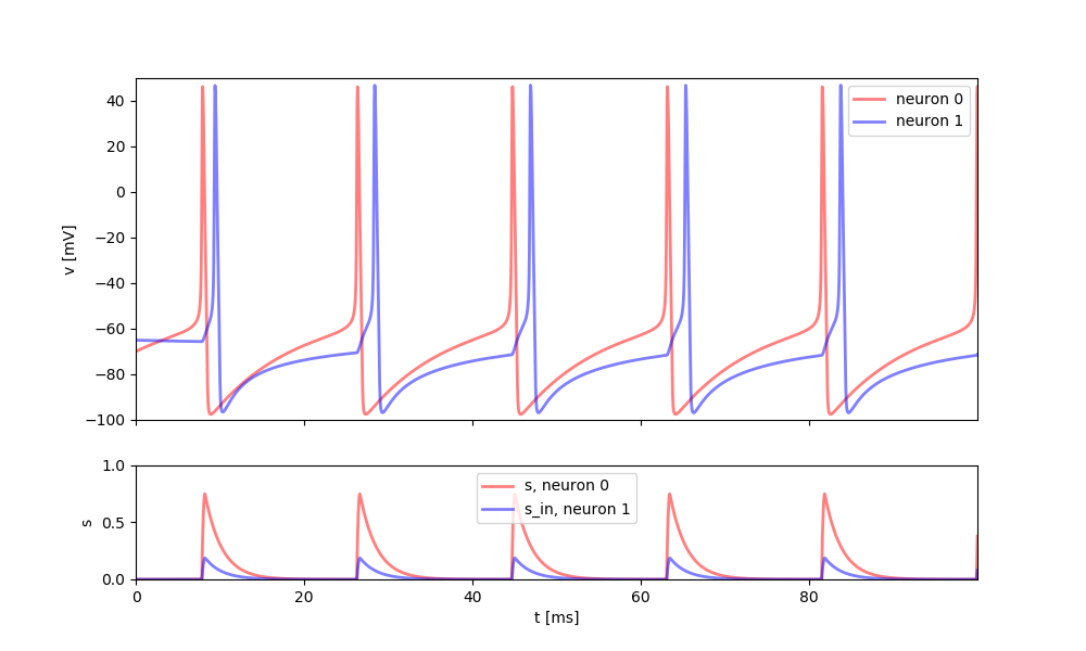
Synaptic model with continuous interaction
This example implements a conductance base synapse that is continuously linking two neurons, i.e. the synaptic gating variable updates at each time step. Two Reduced Traub-Miles Model (RTM) neurons are connected to each other through a directed synapse from neuron 1 to 2.
Here, the complexity stems from the fact that the synaptic conductance is a continuous function of the membrane potential, instead of being triggered by individual spikes. This can be useful in particular when analyzing models mathematically but it is not recommended in most cases because they tend to be less efficient. Also note that this model only works with (pre-synaptic) neuron models that model the action potential in detail, i.e. not with integrate-and-fire type models.
There are two broad approaches (s as part of the pre-synaptic neuron or
s as part of the Synapses object), all depends on whether the time
constants are the same across all synapses or whether they can vary between
synapses. In this example, the time constant is assumed to be the same and
s is therefore part of the pre-synaptic neuron model.
References:
Introduction to modeling neural dynamics, Börgers, chapter 20
from brian2 import *

I_e = 1.5*uA
simulation_time = 100*ms
# neuron RTM parameters
El = -67 * mV
EK = -100 * mV
ENa = 50 * mV
ESyn = 0 * mV
gl = 0.1 * msiemens
gK = 80 * msiemens
gNa = 100 * msiemens

C = 1 * ufarad

weight = 0.25
gSyn = 1.0 * msiemens
tau_d = 2 * ms
tau_r = 0.2 * ms

# forming RTM model with differential equations
eqs = """
alphah = 0.128 * exp(-(vm + 50.0*mV) / (18.0*mV))/ms :Hz
alpham = 0.32/mV * (vm + 54*mV) / (1.0 - exp(-(vm + 54.0*mV) / (4.0*mV)))/ms:Hz
alphan = 0.032/mV * (vm + 52*mV) / (1.0 - exp(-(vm + 52.0*mV) / (5.0*mV)))/ms:Hz

betah  = 4.0 / (1.0 + exp(-(vm + 27.0*mV) / (5.0*mV)))/ms:Hz
betam  = 0.28/mV * (vm + 27.0*mV) / (exp((vm + 27.0*mV) / (5.0*mV)) - 1.0)/ms:Hz
betan  = 0.5 * exp(-(vm + 57.0*mV) / (40.0*mV))/ms:Hz

membrane_Im = I_ext + gNa*m**3*h*(ENa-vm) +
              gl*(El-vm) + gK*n**4*(EK-vm) + gSyn*s_in*(-vm): amp
I_ext : amp
s_in  : 1

dm/dt = alpham*(1-m)-betam*m : 1
dn/dt = alphan*(1-n)-betan*n : 1
dh/dt = alphah*(1-h)-betah*h : 1

ds/dt = 0.5 * (1 + tanh(0.1*vm/mV)) * (1-s)/tau_r - s/tau_d : 1

dvm/dt = membrane_Im/C : volt
"""

neuron = NeuronGroup(2, eqs, method="exponential_euler")

# initialize variables
neuron.vm = [-70.0, -65.0]*mV
neuron.m = "alpham / (alpham + betam)"
neuron.h = "alphah / (alphah + betah)"
neuron.n = "alphan / (alphan + betan)"
neuron.I_ext = [I_e, 0.0*uA]

S = Synapses(neuron,
             neuron,
             's_in_post = weight*s_pre:1 (summed)')
S.connect(i=0, j=1)

# tracking variables
st_mon = StateMonitor(neuron, ["vm", "s", "s_in"], record=[0, 1])

# running the simulation
run(simulation_time)

# plot the results
fig, ax = plt.subplots(2, figsize=(10, 6), sharex=True,
                       gridspec_kw={'height_ratios': (3, 1)})

ax[0].plot(st_mon.t/ms, st_mon.vm[0]/mV,
           lw=2, c="r", alpha=0.5, label="neuron 0")
ax[0].plot(st_mon.t/ms, st_mon.vm[1]/mV,
           lw=2, c="b", alpha=0.5, label='neuron 1')
ax[1].plot(st_mon.t/ms, st_mon.s[0],
           lw=2, c="r", alpha=0.5, label='s, neuron 0')
ax[1].plot(st_mon.t/ms, st_mon.s_in[1],
           lw=2, c="b", alpha=0.5, label='s_in, neuron 1')
ax[0].set(ylabel='v [mV]', xlim=(0, np.max(st_mon.t / ms)),
          ylim=(-100, 50))
ax[1].set(xlabel="t [ms]", ylabel="s", ylim=(0, 1))

ax[0].legend()
ax[1].legend()

plt.show()