Example: Jansen_Rit_1995_single_column
Note
You can launch an interactive, editable version of this example without installing any local files using the Binder service (although note that at some times this may be slow or fail to open):
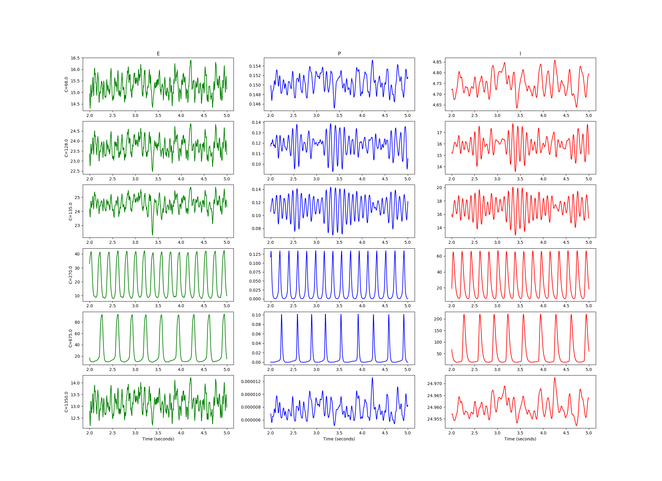
[Jansen and Rit 1995 model](https://link.springer.com/content/pdf/10.1007/BF00199471.pdf) (Figure 3) in Brian2.
Equations are the system of differential equations number (6) in the original paper. The rate parameters $a=100 s^{-1}$ and $b=200 s^{-1}$ were changed to excitatory $tau_e = 1000ms/a =10ms$ and inhibitory $tau_i = 1000ms/b =20ms$ time constants as in [Thomas Knosche review](https://link.springer.com/referenceworkentry/10.1007%2F978-1-4614-6675-8_65), [Touboul et al. 2011](https://direct.mit.edu/neco/article-abstract/23/12/3232/7717/Neural-Mass-Activity-Bifurcations-and-Epilepsy?redirectedFrom=fulltext), or [David & Friston 2003](https://www.sciencedirect.com/science/article/pii/S1053811903004579). Units were removerd from parameters $e_0$, $v_0$, $r_0$, $A$, $B$, and $p$ to stop Brian’s confusion.
Ruben Tikidji-Hamburyan 2021 (rth@r-a-r.org)
from numpy import *
from numpy import random as rnd
from matplotlib.pyplot import *
from brian2 import *

defaultclock.dt = .1*ms   #default time step

te,ti    = 10.*ms, 20.*ms #taus for excitatory and inhibitory populations
e0       = 5.             #max firing rate
v0       = 6.             #(max FR)/2 input
r0       = 0.56           #gain rate
A,B,C    = 3.25, 22., 135 #standard parameters as in the set (7) of the original paper
P,deltaP = 120, 320.-120  #random input uniformly distributed between 120 and
                          #320 pulses per second

# Random noise
nstim = TimedArray(rnd.rand(70000),2*ms)

# Equations as in the system (6) of the original paper
equs = """
dy0/dt = y3                             /second : 1
dy3/dt = (A        * Sp -2*y3 -y0/te*second)/te : 1
dy1/dt = y4                             /second : 1
dy4/dt = (A*(p+ C2 * Se)-2*y4 -y1/te*second)/te : 1
dy2/dt = y5                             /second : 1
dy5/dt = (B   * C4 * Si -2*y5 -y2/ti*second)/ti : 1
p  = P0+nstim(t)*dlP                   : 1
Sp = e0/(1+exp(r0*(v0 - (y1-y2)    ))) : 1
Se = e0/(1+exp(r0*(v0 -  C1*y0     ))) : 1
Si = e0/(1+exp(r0*(v0 -  C3*y0     ))) : 1
C1            : 1
C2 = 0.8 *C1  : 1
C3 = 0.25*C1  : 1
C4 = 0.25*C1  : 1
P0            : 1
dlP           : 1
"""

n = NeuronGroup(6,equs,method='euler') #creates 6 JR models for different connectivity parameters

#set parameters as for different traces on figure 3 of the original paper
n.C1[0]  = 68
n.C1[1]  = 128
n.C1[2]  = C
n.C1[3]  = 270
n.C1[4]  = 675
n.C1[5]  = 1350
#set stimulus offset and noise magnitude
n.P0     = P
n.dlP    = deltaP

#just record everything
sm = StateMonitor(n,['y4','y1','y3','y0','y5','y2'],record=True)

#Runs for 5 second
run(5*second,report='text')


#This code goes over all models with different parameters and plot activity of each population.

figure(1,figsize=(22,16))
idx1 = where(sm.t/second>2.)[0]

o = 0
for p in [0,1,2,3,4,5]:
    if o == 0: ax = subplot(6,3,1)
    else     :subplot(6,3,1+o,sharex=ax)
    if o == 0: title("E")
    plot(sm.t[idx1]/second, sm[p].y1[idx1],'g-')
    ylabel(f"C={n[p].C1[0]}")
    if o == 15: xlabel("Time (seconds)")
    subplot(6,3,2+o,sharex=ax)
    if o == 0: title("P")
    plot(sm.t[idx1]/second, sm[p].y0[idx1],'b-')
    if o == 15: xlabel("Time (seconds)")
    subplot(6,3,3+o,sharex=ax)
    if o == 0: title("I")
    plot(sm.t[idx1]/second, sm[p].y2[idx1],'r-')
    if o == 15: xlabel("Time (seconds)")
    o += 3

show()