Example: stochastic_odes
Note
You can launch an interactive, editable version of this example without installing any local files using the Binder service (although note that at some times this may be slow or fail to open):
Demonstrate the correctness of the “derivative-free Milstein method” for multiplicative noise.
from brian2 import *
# We only get exactly the same random numbers for the exact solution and the
# simulation if we use the numpy code generation target
prefs.codegen.target = 'numpy'
# setting a random seed makes all variants use exactly the same Wiener process
seed = 12347
X0 = 1
mu = 0.5/second # drift
sigma = 0.1/second #diffusion
runtime = 1*second
def simulate(method, dt):
"""
simulate geometrical Brownian with the given method
"""
np.random.seed(seed)
G = NeuronGroup(1, 'dX/dt = (mu - 0.5*second*sigma**2)*X + X*sigma*xi*second**.5: 1',
dt=dt, method=method)
G.X = X0
mon = StateMonitor(G, 'X', record=True)
net = Network(G, mon)
net.run(runtime)
return mon.t_[:], mon.X.flatten()
def exact_solution(t, dt):
"""
Return the exact solution for geometrical Brownian motion at the given
time points
"""
# Remove units for simplicity
my_mu = float(mu)
my_sigma = float(sigma)
dt = float(dt)
t = asarray(t)
np.random.seed(seed)
# We are calculating the values at the *start* of a time step, as when using
# a StateMonitor. Therefore the Brownian motion starts with zero
brownian = np.hstack([0, cumsum(sqrt(dt) * np.random.randn(len(t)-1))])
return (X0 * exp((my_mu - 0.5*my_sigma**2)*(t+dt) + my_sigma*brownian))
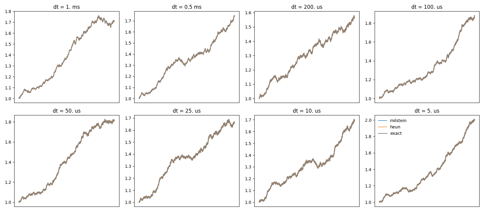
figure(1, figsize=(16, 7))
figure(2, figsize=(16, 7))
methods = ['milstein', 'heun']
dts = [1*ms, 0.5*ms, 0.2*ms, 0.1*ms, 0.05*ms, 0.025*ms, 0.01*ms, 0.005*ms]
rows = int(sqrt(len(dts)))
cols = int(ceil(1.0 * len(dts) / rows))
errors = dict([(method, zeros(len(dts))) for method in methods])
for dt_idx, dt in enumerate(dts):
print('dt: %s' % dt)
trajectories = {}
# Test the numerical methods
for method in methods:
t, trajectories[method] = simulate(method, dt)
# Calculate the exact solution
exact = exact_solution(t, dt)
for method in methods:
# plot the trajectories
figure(1)
subplot(rows, cols, dt_idx+1)
plot(t, trajectories[method], label=method, alpha=0.75)
# determine the mean absolute error
errors[method][dt_idx] = mean(abs(trajectories[method] - exact))
# plot the difference to the real trajectory
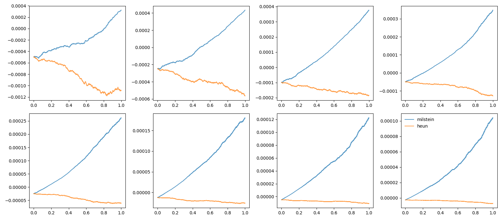
figure(2)
subplot(rows, cols, dt_idx+1)
plot(t, trajectories[method] - exact, label=method, alpha=0.75)
figure(1)
plot(t, exact, color='gray', lw=2, label='exact', alpha=0.75)
title('dt = %s' % str(dt))
xticks([])
figure(1)
legend(frameon=False, loc='best')
tight_layout()
figure(2)
legend(frameon=False, loc='best')
tight_layout()
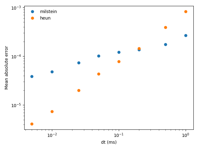
figure(3)
for method in methods:
plot(array(dts) / ms, errors[method], 'o', label=method)
legend(frameon=False, loc='best')
xscale('log')
yscale('log')
xlabel('dt (ms)')
ylabel('Mean absolute error')
tight_layout()
show()