Example: example_2_gchi_astrocyte
Note
You can launch an interactive, editable version of this example without installing any local files using the Binder service (although note that at some times this may be slow or fail to open):
Modeling neuron-glia interactions with the Brian 2 simulator Marcel Stimberg, Dan F. M. Goodman, Romain Brette, Maurizio De Pittà bioRxiv 198366; doi: https://doi.org/10.1101/198366
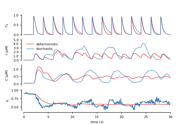
Figure 2: Modeling of synaptically-activated astrocytes
Two astrocytes (one stochastic and the other deterministic) activated by synapses (connecting “dummy” groups of neurons) (see De Pitta’ et al., 2009)
from brian2 import *

import plot_utils as pu

set_device('cpp_standalone', directory=None)  # Use fast "C++ standalone mode"
seed(790824)  # to get identical figures for repeated runs

################################################################################
# Model parameters
################################################################################
### General parameters
duration = 30*second          # Total simulation time
sim_dt = 1*ms                 # Integrator/sampling step

### Neuron parameters
f_0 = 0.5*Hz                  # Spike rate of the "source" neurons

### Synapse parameters
rho_c = 0.001                 # Synaptic vesicle-to-extracellular space volume ratio
Y_T = 500*mmolar              # Total vesicular neurotransmitter concentration
Omega_c = 40/second           # Neurotransmitter clearance rate

### Astrocyte parameters
# ---  Calcium fluxes
O_P = 0.9*umolar/second       # Maximal Ca^2+ uptake rate by SERCAs
K_P = 0.1 * umolar            # Ca2+ affinity of SERCAs
C_T = 2*umolar                # Total cell free Ca^2+ content
rho_A = 0.18                  # ER-to-cytoplasm volume ratio
Omega_C = 6/second            # Maximal rate of Ca^2+ release by IP_3Rs
Omega_L = 0.1/second          # Maximal rate of Ca^2+ leak from the ER
# --- IP_3R kinectics
d_1 = 0.13*umolar             # IP_3 binding affinity
d_2 = 1.05*umolar             # Ca^2+ inactivation dissociation constant
O_2 = 0.2/umolar/second       # IP_3R binding rate for Ca^2+ inhibition
d_3 = 0.9434*umolar           # IP_3 dissociation constant
d_5 = 0.08*umolar             # Ca^2+ activation dissociation constant
# --- Agonist-dependent IP_3 production
O_beta = 5*umolar/second      # Maximal rate of IP_3 production by PLCbeta
O_N = 0.3/umolar/second       # Agonist binding rate
Omega_N = 0.5/second          # Maximal inactivation rate
K_KC = 0.5*umolar             # Ca^2+ affinity of PKC
zeta = 10                     # Maximal reduction of receptor affinity by PKC
# --- IP_3 production
O_delta = 0.2 *umolar/second  # Maximal rate of IP_3 production by PLCdelta
kappa_delta = 1.5 * umolar    # Inhibition constant of PLC_delta by IP_3
K_delta = 0.3*umolar          # Ca^2+ affinity of PLCdelta
# --- IP_3 degradation
Omega_5P = 0.1/second         # Maximal rate of IP_3 degradation by IP-5P
K_D = 0.5*umolar              # Ca^2+ affinity of IP3-3K
K_3K = 1*umolar               # IP_3 affinity of IP_3-3K
O_3K = 4.5*umolar/second      # Maximal rate of IP_3 degradation by IP_3-3K
# --- IP_3 external production
F_ex = 0.09*umolar/second     # Maximal exogenous IP3 flow
I_Theta = 0.3*umolar          # Threshold gradient for IP_3 diffusion
omega_I = 0.05*umolar         # Scaling factor of diffusion

################################################################################
# Model definition
################################################################################
defaultclock.dt = sim_dt  # Set the integration time

### "Neurons"
# (We are only interested in the activity of the synapse, so we replace the
# neurons by trivial "dummy" groups
# # Regular spiking neuron
source_neurons = NeuronGroup(1, 'dx/dt = f_0 : 1', threshold='x>1',
                             reset='x=0', method='euler')
## Dummy neuron
target_neurons = NeuronGroup(1, '')


### Synapses
# Our synapse model is trivial, we are only interested in its neurotransmitter
# release
synapses_eqs = 'dY_S/dt = -Omega_c * Y_S : mmolar (clock-driven)'
synapses_action = 'Y_S += rho_c * Y_T'
synapses = Synapses(source_neurons, target_neurons,
                    model=synapses_eqs, on_pre=synapses_action,
                    method='exact')
synapses.connect()

### Astrocytes
# We are modelling two astrocytes, the first is deterministic while the second
# displays stochastic dynamics
astro_eqs = '''
# Fraction of activated astrocyte receptors:
dGamma_A/dt = O_N * Y_S * (1 - Gamma_A) -
              Omega_N*(1 + zeta * C/(C + K_KC)) * Gamma_A : 1

# IP_3 dynamics:
dI/dt = J_beta + J_delta - J_3K - J_5P + J_ex     : mmolar
J_beta = O_beta * Gamma_A                         : mmolar/second
J_delta = O_delta/(1 + I/kappa_delta) *
                         C**2/(C**2 + K_delta**2) : mmolar/second
J_3K = O_3K * C**4/(C**4 + K_D**4) * I/(I + K_3K) : mmolar/second
J_5P = Omega_5P*I                                 : mmolar/second
delta_I_bias = I - I_bias : mmolar
J_ex = -F_ex/2*(1 + tanh((abs(delta_I_bias) - I_Theta)/omega_I)) *
                sign(delta_I_bias)                : mmolar/second
I_bias                                            : mmolar (constant)

# Ca^2+-induced Ca^2+ release:
dC/dt = J_r + J_l - J_p                : mmolar
# IP3R de-inactivation probability
dh/dt = (h_inf - h_clipped)/tau_h *
        (1 + noise*xi*tau_h**0.5)      : 1
h_clipped = clip(h,0,1)                : 1
J_r = (Omega_C * m_inf**3 * h_clipped**3) *
      (C_T - (1 + rho_A)*C)            : mmolar/second
J_l = Omega_L * (C_T - (1 + rho_A)*C)  : mmolar/second
J_p = O_P * C**2/(C**2 + K_P**2)       : mmolar/second
m_inf = I/(I + d_1) * C/(C + d_5)      : 1
h_inf = Q_2/(Q_2 + C)                  : 1
tau_h = 1/(O_2 * (Q_2 + C))            : second
Q_2 = d_2 * (I + d_1)/(I + d_3)        : mmolar

# Neurotransmitter concentration in the extracellular space
Y_S     : mmolar
# Noise flag
noise   : 1 (constant)
'''
# Milstein integration method for the multiplicative noise
astrocytes = NeuronGroup(2, astro_eqs, method='milstein')
astrocytes.h = 0.9  # IP3Rs are initially mostly available for CICR

# The first astrocyte is deterministic ("zero noise"), the second stochastic
astrocytes.noise = [0, 1]
# Connection between synapses and astrocytes (both astrocytes receive the
# same input from the synapse). Note that in this special case, where each
# astrocyte is only influenced by the neurotransmitter from a single synapse,
# the '(linked)' variable mechanism could be used instead. The mechanism used
# below is more general and can add the contribution of several synapses.
ecs_syn_to_astro = Synapses(synapses, astrocytes,
                            'Y_S_post = Y_S_pre : mmolar (summed)')
ecs_syn_to_astro.connect()
################################################################################
# Monitors
################################################################################
astro_mon = StateMonitor(astrocytes, variables=['Gamma_A', 'C', 'h', 'I'],
                         record=True)

################################################################################
# Simulation run
################################################################################
run(duration, report='text')

################################################################################
# Analysis and plotting
################################################################################
from matplotlib.ticker import FormatStrFormatter
plt.style.use('figures.mplstyle')

# Plot Gamma_A
fig, ax = plt.subplots(4, 1, figsize=(6.26894, 6.26894*0.66))
ax[0].plot(astro_mon.t/second, astro_mon.Gamma_A.T)
ax[0].set(xlim=(0., duration/second), ylim=[-0.05, 1.02], yticks=[0.0, 0.5, 1.0],
          ylabel=r'$\Gamma_{A}$')
# Adjust axis
pu.adjust_spines(ax[0], ['left'])

# Plot I
ax[1].plot(astro_mon.t/second, astro_mon.I.T/umolar)
ax[1].set(xlim=(0., duration/second), ylim=[-0.1, 5.0],
          yticks=arange(0.0, 5.1, 1., dtype=float),
          ylabel=r'$I$ ($\mu M$)')
ax[1].yaxis.set_major_formatter(FormatStrFormatter('%.1f'))
ax[1].legend(['deterministic', 'stochastic'], loc='upper left')
pu.adjust_spines(ax[1], ['left'])

# Plot C
ax[2].plot(astro_mon.t/second, astro_mon.C.T/umolar)
ax[2].set(xlim=(0., duration/second), ylim=[-0.1, 1.3],
          ylabel=r'$C$ ($\mu M$)')
pu.adjust_spines(ax[2], ['left'])

# Plot h
ax[3].plot(astro_mon.t/second, astro_mon.h.T)
ax[3].set(xlim=(0., duration/second),
          ylim=[0.4, 1.02],
          ylabel='h', xlabel='time ($s$)')
pu.adjust_spines(ax[3], ['left', 'bottom'])

pu.adjust_ylabels(ax, x_offset=-0.1)

plt.show()