Example: example_5_astro_ring
Note
You can launch an interactive, editable version of this example without installing any local files using the Binder service (although note that at some times this may be slow or fail to open):
Modeling neuron-glia interactions with the Brian 2 simulator Marcel Stimberg, Dan F. M. Goodman, Romain Brette, Maurizio De Pittà bioRxiv 198366; doi: https://doi.org/10.1101/198366
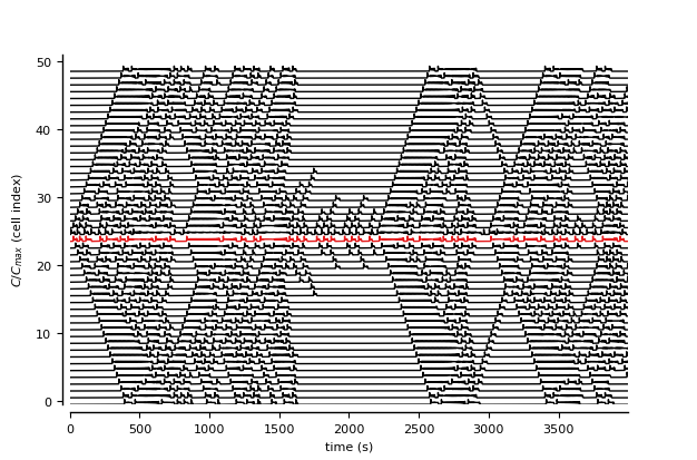
Figure 5: Astrocytes connected in a network.
Intercellular calcium wave propagation in a ring of 50 astrocytes connected by bidirectional gap junctions (see Goldberg et al., 2010)
from brian2 import *

import plot_utils as pu

set_device('cpp_standalone', directory=None)  # Use fast "C++ standalone mode"

################################################################################
# Model parameters
################################################################################
### General parameters
duration = 4000*second       # Total simulation time
sim_dt = 50*ms               # Integrator/sampling step

### Astrocyte parameters
# ---  Calcium fluxes
O_P = 0.9*umolar/second      # Maximal Ca^2+ uptake rate by SERCAs
K_P = 0.05 * umolar          # Ca2+ affinity of SERCAs
C_T = 2*umolar               # Total cell free Ca^2+ content
rho_A = 0.18                 # ER-to-cytoplasm volume ratio
Omega_C = 6/second           # Maximal rate of Ca^2+ release by IP_3Rs
Omega_L = 0.1/second         # Maximal rate of Ca^2+ leak from the ER
# --- IP_3R kinectics
d_1 = 0.13*umolar            # IP_3 binding affinity
d_2 = 1.05*umolar            # Ca^2+ inactivation dissociation constant
O_2 = 0.2/umolar/second      # IP_3R binding rate for Ca^2+ inhibition
d_3 = 0.9434*umolar          # IP_3 dissociation constant
d_5 = 0.08*umolar            # Ca^2+ activation dissociation constant
# --- IP_3 production
O_delta = 0.6*umolar/second  # Maximal rate of IP_3 production by PLCdelta
kappa_delta = 1.5* umolar    # Inhibition constant of PLC_delta by IP_3
K_delta = 0.1*umolar         # Ca^2+ affinity of PLCdelta
# --- IP_3 degradation
Omega_5P = 0.05/second       # Maximal rate of IP_3 degradation by IP-5P
K_D = 0.7*umolar             # Ca^2+ affinity of IP3-3K
K_3K = 1.0*umolar            # IP_3 affinity of IP_3-3K
O_3K = 4.5*umolar/second     # Maximal rate of IP_3 degradation by IP_3-3K
# --- IP_3 diffusion
F_ex = 0.09*umolar/second    # Maximal exogenous IP3 flow
F = 0.09*umolar/second       # GJC IP_3 permeability
I_Theta = 0.3*umolar         # Threshold gradient for IP_3 diffusion
omega_I = 0.05*umolar        # Scaling factor of diffusion

################################################################################
# Model definition
################################################################################
defaultclock.dt = sim_dt     # Set the integration time

### Astrocytes
astro_eqs = '''
dI/dt = J_delta - J_3K - J_5P + J_ex + J_coupling : mmolar
J_delta = O_delta/(1 + I/kappa_delta) * C**2/(C**2 + K_delta**2) : mmolar/second
J_3K = O_3K * C**4/(C**4 + K_D**4) * I/(I + K_3K)                : mmolar/second
J_5P = Omega_5P*I                                                : mmolar/second
# Exogenous stimulation (rectangular wave with period of 50s and duty factor 0.4)
stimulus = int((t % (50*second))<20*second)                      : 1
delta_I_bias = I - I_bias*stimulus                               : mmolar
J_ex = -F_ex/2*(1 + tanh((abs(delta_I_bias) - I_Theta)/omega_I)) *
                sign(delta_I_bias)                               : mmolar/second
# Diffusion between astrocytes
J_coupling : mmolar/second

# Ca^2+-induced Ca^2+ release:
dC/dt = J_r + J_l - J_p                                   : mmolar
dh/dt = (h_inf - h)/tau_h                                 : 1
J_r = (Omega_C * m_inf**3 * h**3) * (C_T - (1 + rho_A)*C) : mmolar/second
J_l = Omega_L * (C_T - (1 + rho_A)*C)                     : mmolar/second
J_p = O_P * C**2/(C**2 + K_P**2)                          : mmolar/second
m_inf = I/(I + d_1) * C/(C + d_5)                         : 1
h_inf = Q_2/(Q_2 + C)                                     : 1
tau_h = 1/(O_2 * (Q_2 + C))                               : second
Q_2 = d_2 * (I + d_1)/(I + d_3)                           : mmolar

# External IP_3 drive
I_bias : mmolar (constant)
'''

N_astro = 50 # Total number of astrocytes in the network
astrocytes = NeuronGroup(N_astro, astro_eqs, method='rk4')
# Asymmetric stimulation on the 50th cell to get some nice chaotic patterns
astrocytes.I_bias[N_astro//2] = 1.0*umolar
astrocytes.h = 0.9
# Diffusion between astrocytes
astro_to_astro_eqs = '''
delta_I = I_post - I_pre        : mmolar
J_coupling_post = -F/2 * (1 + tanh((abs(delta_I) - I_Theta)/omega_I)) *
                  sign(delta_I) : mmolar/second (summed)
'''
astro_to_astro = Synapses(astrocytes, astrocytes,
                          model=astro_to_astro_eqs)
# Couple neighboring astrocytes: two connections per astrocyte pair, as
# the above formulation will only update the I_coupling term of one of the
# astrocytes
astro_to_astro.connect('j == (i + 1) % N_pre or '
                       'j == (i + N_pre - 1) % N_pre')

################################################################################
# Monitors
################################################################################
astro_mon = StateMonitor(astrocytes, variables=['C'], record=True)

################################################################################
# Simulation run
################################################################################
run(duration, report='text')

################################################################################
# Analysis and plotting
################################################################################
plt.style.use('figures.mplstyle')

fig, ax = plt.subplots(nrows=1, ncols=1, figsize=(6.26894, 6.26894 * 0.66),
                       gridspec_kw={'left': 0.1, 'bottom': 0.12})
scaling = 1.2
step = 10
ax.plot(astro_mon.t/second,
        (astro_mon.C[0:N_astro//2-1].T/astro_mon.C.max() +
         np.arange(N_astro//2-1)*scaling), color='black')
ax.plot(astro_mon.t/second, (astro_mon.C[N_astro//2:].T/astro_mon.C.max() +
                             np.arange(N_astro//2, N_astro)*scaling),
        color='black')
ax.plot(astro_mon.t/second, (astro_mon.C[N_astro//2-1].T/astro_mon.C.max() +
                             np.arange(N_astro//2-1, N_astro//2)*scaling),
        color='C0')
ax.set(xlim=(0., duration/second), ylim=(0, (N_astro+1.5)*scaling),
       xticks=np.arange(0., duration/second, 500), xlabel='time (s)',
       yticks=np.arange(0.5*scaling, (N_astro + 1.5)*scaling, step*scaling),
       yticklabels=[str(yt) for yt in np.arange(0, N_astro + 1, step)],
       ylabel='$C/C_{max}$ (cell index)')
pu.adjust_spines(ax, ['left', 'bottom'])

pu.adjust_ylabels([ax], x_offset=-0.08)

plt.show()