Example: hodgkin_huxley_1952
Note
You can launch an interactive, editable version of this example without installing any local files using the Binder service (although note that at some times this may be slow or fail to open):
Hodgkin-Huxley equations (1952).
from brian2 import *
morpho = Cylinder(length=10*cm, diameter=2*238*um, n=1000, type='axon')
El = 10.613*mV
ENa = 115*mV
EK = -12*mV
gl = 0.3*msiemens/cm**2
gNa0 = 120*msiemens/cm**2
gK = 36*msiemens/cm**2
# Typical equations
eqs = '''
# The same equations for the whole neuron, but possibly different parameter values
# distributed transmembrane current
Im = gl * (El-v) + gNa * m**3 * h * (ENa-v) + gK * n**4 * (EK-v) : amp/meter**2
I : amp (point current) # applied current
dm/dt = alpham * (1-m) - betam * m : 1
dn/dt = alphan * (1-n) - betan * n : 1
dh/dt = alphah * (1-h) - betah * h : 1
alpham = (0.1/mV) * 10*mV/exprel((-v+25*mV)/(10*mV))/ms : Hz
betam = 4 * exp(-v/(18*mV))/ms : Hz
alphah = 0.07 * exp(-v/(20*mV))/ms : Hz
betah = 1/(exp((-v+30*mV) / (10*mV)) + 1)/ms : Hz
alphan = (0.01/mV) * 10*mV/exprel((-v+10*mV)/(10*mV))/ms : Hz
betan = 0.125*exp(-v/(80*mV))/ms : Hz
gNa : siemens/meter**2
'''
neuron = SpatialNeuron(morphology=morpho, model=eqs, Cm=1*uF/cm**2,
Ri=35.4*ohm*cm, method="exponential_euler")
neuron.v = 0*mV
neuron.h = 1
neuron.m = 0
neuron.n = .5
neuron.I = 0
neuron.gNa = gNa0
neuron[5*cm:10*cm].gNa = 0*siemens/cm**2
M = StateMonitor(neuron, 'v', record=True)
run(50*ms, report='text')
neuron.I[0] = 1*uA # current injection at one end
run(3*ms)
neuron.I = 0*amp
run(100*ms, report='text')
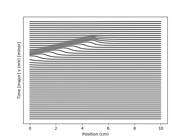
for i in range(75, 125, 1):
plot(cumsum(neuron.length)/cm, i+(1./60)*M.v[:, i*5]/mV, 'k')
yticks([])
ylabel('Time [major] v (mV) [minor]')
xlabel('Position (cm)')
axis('tight')
show()