Example: example_4_rsmean
Note
You can launch an interactive, editable version of this example without installing any local files using the Binder service (although note that at some times this may be slow or fail to open):
Modeling neuron-glia interactions with the Brian 2 simulator Marcel Stimberg, Dan F. M. Goodman, Romain Brette, Maurizio De Pittà bioRxiv 198366; doi: https://doi.org/10.1101/198366
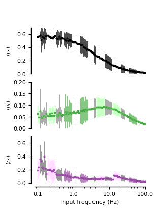
Figure 4C: Closed-loop gliotransmission.
I/O curves in terms average per-spike release vs. rate of stimulation for three synapses: one without gliotransmission, and the other two with open- and close-loop gliotransmssion.
from brian2 import *

import plot_utils as pu

set_device('cpp_standalone', directory=None)  # Use fast "C++ standalone mode"
seed(1929)  # to get identical figures for repeated runs

################################################################################
# Model parameters
################################################################################
### General parameters
N_synapses = 100
N_astro = 2
transient = 15*second
duration = transient + 180*second  # Total simulation time
sim_dt = 1*ms                      # Integrator/sampling step

### Neuron parameters

# ### Synapse parameters
### Synapse parameters
rho_c = 0.005               # Synaptic vesicle-to-extracellular space volume ratio
Y_T = 500*mmolar            # Total vesicular neurotransmitter concentration
Omega_c = 40/second         # Neurotransmitter clearance rate
U_0__star = 0.6             # Resting synaptic release probability
Omega_f = 3.33/second       # Synaptic facilitation rate
Omega_d = 2.0/second        # Synaptic depression rate
# --- Presynaptic receptors
O_G = 1.5/umolar/second     # Agonist binding (activating) rate
Omega_G = 0.5/(60*second)   # Agonist release (deactivating) rate

### Astrocyte parameters
# ---  Calcium fluxes
O_P = 0.9*umolar/second     # Maximal Ca^2+ uptake rate by SERCAs
K_P = 0.05 * umolar         # Ca2+ affinity of SERCAs
C_T = 2*umolar              # Total cell free Ca^2+ content
rho_A = 0.18                # ER-to-cytoplasm volume ratio
Omega_C = 6/second          # Maximal rate of Ca^2+ release by IP_3Rs
Omega_L = 0.1/second        # Maximal rate of Ca^2+ leak from the ER
# --- IP_3R kinectics
d_1 = 0.13*umolar           # IP_3 binding affinity
d_2 = 1.05*umolar           # Ca^2+ inactivation dissociation constant
O_2 = 0.2/umolar/second     # IP_3R binding rate for Ca^2+ inhibition
d_3 = 0.9434*umolar         # IP_3 dissociation constant
d_5 = 0.08*umolar           # Ca^2+ activation dissociation constant
# --- IP_3 production
# --- Agonist-dependent IP_3 production
O_beta = 3.2*umolar/second  # Maximal rate of IP_3 production by PLCbeta
O_N = 0.3/umolar/second     # Agonist binding rate
Omega_N = 0.5/second        # Maximal inactivation rate
K_KC = 0.5*umolar           # Ca^2+ affinity of PKC
zeta = 10                   # Maximal reduction of receptor affinity by PKC
# --- Endogenous IP3 production
O_delta = 0.6*umolar/second # Maximal rate of IP_3 production by PLCdelta
kappa_delta = 1.5* umolar   # Inhibition constant of PLC_delta by IP_3
K_delta = 0.1*umolar        # Ca^2+ affinity of PLCdelta
# --- IP_3 degradation
Omega_5P = 0.05/second      # Maximal rate of IP_3 degradation by IP-5P
K_D = 0.7*umolar            # Ca^2+ affinity of IP3-3K
K_3K = 1.0*umolar           # IP_3 affinity of IP_3-3K
O_3K = 4.5*umolar/second    # Maximal rate of IP_3 degradation by IP_3-3K
# --- IP_3 diffusion
F_ex = 2.0*umolar/second    # Maximal exogenous IP3 flow
I_Theta = 0.3*umolar        # Threshold gradient for IP_3 diffusion
omega_I = 0.05*umolar       # Scaling factor of diffusion
# --- Gliotransmitter release and time course
C_Theta = 0.5*umolar        # Ca^2+ threshold for exocytosis
Omega_A = 0.6/second        # Gliotransmitter recycling rate
U_A = 0.6                   # Gliotransmitter release probability
G_T = 200*mmolar            # Total vesicular gliotransmitter concentration
rho_e = 6.5e-4              # Astrocytic vesicle-to-extracellular volume ratio
Omega_e = 60/second         # Gliotransmitter clearance rate
alpha = 0.0                 # Gliotransmission nature

################################################################################
# Model definition
################################################################################
defaultclock.dt = sim_dt  # Set the integration time

f_vals = np.logspace(-1, 2, N_synapses)*Hz
source_neurons = PoissonGroup(N_synapses, rates=f_vals)
target_neurons = NeuronGroup(N_synapses, '')

### Synapses
# Note that the synapse does not actually have any effect on the post-synaptic
# target
# Also note that for easier plotting we do not use the "event-driven" flag here,
# even though the value of u_S and x_S only needs to be updated on the arrival
# of a spike
synapses_eqs = '''
# Neurotransmitter
dY_S/dt = -Omega_c * Y_S : mmolar (clock-driven)
# Fraction of activated presynaptic receptors
dGamma_S/dt = O_G * G_A * (1 - Gamma_S) - Omega_G * Gamma_S : 1 (clock-driven)
# Usage of releasable neurotransmitter per single action potential:
du_S/dt = -Omega_f * u_S : 1 (event-driven)
# Fraction of synaptic neurotransmitter resources available for release:
dx_S/dt = Omega_d *(1 - x_S) : 1 (event-driven)
r_S : 1  # released synaptic neurotransmitter resources
G_A : mmolar  # gliotransmitter concentration in the extracellular space
'''
synapses_action = '''
U_0 = (1 - Gamma_S) * U_0__star + alpha * Gamma_S
u_S += U_0 * (1 - u_S)
r_S = u_S * x_S
x_S -= r_S
Y_S += rho_c * Y_T * r_S
'''
synapses = Synapses(source_neurons, target_neurons,
                    model=synapses_eqs, on_pre=synapses_action,
                    method='exact')
# We create three synapses per connection: only the first two are modulated by
# the astrocyte however. Note that we could also create three synapses per
# connection with a single connect call by using connect(j='i', n=3), but this
# would create synapses arranged differently (synapses connection pairs
# (0, 0), (0, 0), (0, 0), (1, 1), (1, 1), (1, 1), ..., instead of
# connections (0, 0), (1, 1), ..., (0, 0), (1, 1), ..., (0, 0), (1, 1), ...)
# making the later connection descriptions more complicated.
synapses.connect(j='i')  # closed-loop modulation
synapses.connect(j='i')  # open modulation
synapses.connect(j='i')  # no modulation
synapses.x_S = 1.0

### Astrocytes
# The astrocyte emits gliotransmitter when its Ca^2+ concentration crosses
# a threshold
astro_eqs = '''
# Fraction of activated astrocyte receptors:
dGamma_A/dt = O_N * Y_S * (1 - Gamma_A) -
              Omega_N*(1 + zeta * C/(C + K_KC)) * Gamma_A : 1

# IP_3 dynamics:
dI/dt = J_beta + J_delta - J_3K - J_5P + J_ex             : mmolar
J_beta = O_beta * Gamma_A                                 : mmolar/second
J_delta = O_delta/(1 + I/kappa_delta) *
                         C**2/(C**2 + K_delta**2)         : mmolar/second
J_3K = O_3K * C**4/(C**4 + K_D**4) * I/(I + K_3K)         : mmolar/second
J_5P = Omega_5P*I                                         : mmolar/second
delta_I_bias = I - I_bias : mmolar
J_ex = -F_ex/2*(1 + tanh((abs(delta_I_bias) - I_Theta)/omega_I)) *
                sign(delta_I_bias)                        : mmolar/second
I_bias                                                    : mmolar (constant)

# Ca^2+-induced Ca^2+ release:
dC/dt = (Omega_C * m_inf**3 * h**3 + Omega_L) * (C_T - (1 + rho_A)*C) -
        O_P * C**2/(C**2 + K_P**2) : mmolar
dh/dt = (h_inf - h)/tau_h          : 1  # IP3R de-inactivation probability
m_inf = I/(I + d_1) * C/(C + d_5)  : 1
h_inf = Q_2/(Q_2 + C)              : 1
tau_h = 1/(O_2 * (Q_2 + C))        : second
Q_2 = d_2 * (I + d_1)/(I + d_3)    : mmolar

# Fraction of gliotransmitter resources available for release
dx_A/dt = Omega_A * (1 - x_A) : 1
# gliotransmitter concentration in the extracellular space
dG_A/dt = -Omega_e*G_A        : mmolar
# Neurotransmitter concentration in the extracellular space
Y_S                           : mmolar
'''
glio_release = '''
G_A += rho_e * G_T * U_A * x_A
x_A -= U_A *  x_A
'''
astrocyte = NeuronGroup(N_astro*N_synapses, astro_eqs,
                        # The following formulation makes sure that a "spike" is
                        # only triggered at the first threshold crossing
                        threshold='C>C_Theta',
                        refractory='C>C_Theta',
                        # The gliotransmitter release happens when the threshold
                        # is crossed, in Brian terms it can therefore be
                        # considered a "reset"
                        reset=glio_release,
                        method='rk4')
astrocyte.h = 0.9
astrocyte.x_A = 1.0
# Only the second group of N_synapses astrocytes are activated by external stimulation
astrocyte.I_bias = (np.r_[np.zeros(N_synapses), np.ones(N_synapses)])*1.0*umolar

## Connections
ecs_syn_to_astro = Synapses(synapses, astrocyte,
                            'Y_S_post = Y_S_pre : mmolar (summed)')
# Connect the first N_synapses synapses--astrocyte pairs
ecs_syn_to_astro.connect(j='i if i < N_synapses')

ecs_astro_to_syn = Synapses(astrocyte, synapses,
                            'G_A_post = G_A_pre : mmolar (summed)')
# Connect the first N_synapses astrocytes--pairs
# (closed-loop configuration)
ecs_astro_to_syn.connect(j='i if i < N_synapses')
# Connect the second N_synapses astrocyte--synapses pairs
# (open-loop configuration)
ecs_astro_to_syn.connect(j='i if i >= N_synapses and i < 2*N_synapses')

################################################################################
# Monitors
################################################################################
syn_mon = StateMonitor(synapses, 'r_S',
                       record=np.arange(N_synapses*(N_astro+1)))

################################################################################
# Simulation run
################################################################################
run(duration, report='text')

################################################################################
# Analysis and plotting
################################################################################
plt.style.use('figures.mplstyle')

fig, ax = plt.subplots(nrows=4, ncols=1, figsize=(3.07, 3.07*1.33), sharex=False,
                       gridspec_kw={'height_ratios': [1, 3, 3, 3],
                                    'top': 0.98, 'bottom': 0.12,
                                    'left': 0.22, 'right': 0.93})

## Turn off one axis to display accordingly to the other figure in example_4_synrel.py
ax[0].axis('off')

ax[1].errorbar(f_vals/Hz, np.mean(syn_mon.r_S[2*N_synapses:], axis=1),
               np.std(syn_mon.r_S[2*N_synapses:], axis=1),
               fmt='o', color='black', lw=0.5)
ax[1].set(xlim=(0.08, 100), xscale='log',
          ylim=(0., 0.7),
          ylabel=r'$\langle r_S \rangle$')
pu.adjust_spines(ax[1], ['left'])

ax[2].errorbar(f_vals/Hz, np.mean(syn_mon.r_S[N_synapses:2*N_synapses], axis=1),
               np.std(syn_mon.r_S[N_synapses:2*N_synapses], axis=1),
               fmt='o', color='C2', lw=0.5)
ax[2].set(xlim=(0.08, 100), xscale='log',
          ylim=(0., 0.2), ylabel=r'$\langle r_S \rangle$')
pu.adjust_spines(ax[2], ['left'])

ax[3].errorbar(f_vals/Hz, np.mean(syn_mon.r_S[:N_synapses], axis=1),
               np.std(syn_mon.r_S[:N_synapses], axis=1),
               fmt='o', color='C3', lw=0.5)
ax[3].set(xlim=(0.08, 100), xticks=np.logspace(-1, 2, 4), xscale='log',
          ylim=(0., 0.7), xlabel='input frequency (Hz)',
          ylabel=r'$\langle r_S \rangle$')
ax[3].xaxis.set_major_formatter(ScalarFormatter())
pu.adjust_spines(ax[3], ['left', 'bottom'])

pu.adjust_ylabels(ax, x_offset=-0.2)

plt.show()