Example: compare_GSL_to_conventional
Note
You can launch an interactive, editable version of this example without installing any local files using the Binder service (although note that at some times this may be slow or fail to open):
Example using GSL ODE solvers with a variable time step and comparing it to the Brian solver.
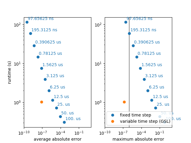
For highly accurate simulations, i.e. simulations with a very low desired error, the GSL simulation with a variable time step can be faster because it uses a low time step only when it is necessary. In biologically detailed models (e.g. of the Hodgkin-Huxley type), the relevant time constants are very short around an action potential, but much longer when the neuron is near its resting potential. The following example uses a very simple neuron model (leaky integrate-and-fire), but simulates a change in relevant time constants by changing the actual time constant every 10ms, independently for each of 100 neurons. To accurately simulate this model with a fixed time step, the time step has to be very small, wasting many unnecessary steps for all the neurons where the time constant is long.
Note that using the GSL ODE solver is much slower, if both methods use a comparable number of steps, i.e. if the desired accuracy is low enough so that a single step per “Brian time step” is enough.
from brian2 import *
import time

# Run settings
start_dt = .1 * ms
method = 'rk2'
error = 1.e-6  # requested accuracy


def runner(method, dt, options=None):
    seed(0)
    I = 5
    group = NeuronGroup(100, '''dv/dt = (-v + I)/tau : 1
                                tau : second''',
                        method=method,
                        method_options=options,
                        dt=dt)
    group.run_regularly('''v = rand()
                           tau = 0.1*ms + rand()*9.9*ms''', dt=10*ms)

    rec_vars = ['v', 'tau']
    if 'gsl' in method:
        rec_vars += ['_step_count']
    net = Network(group)
    net.run(0 * ms)
    mon = StateMonitor(group, rec_vars, record=True, dt=start_dt)
    net.add(mon)
    start = time.time()
    net.run(1 * second)
    mon.add_attribute('run_time')
    mon.run_time = time.time() - start
    return mon


lin = runner('linear', start_dt)
method_options = {'save_step_count': True,
                  'absolute_error': error,
                  'max_steps': 10000}
gsl = runner('gsl_%s' % method, start_dt, options=method_options)

print("Running with GSL integrator and variable time step:")
print('Run time: %.3fs' % gsl.run_time)

# check gsl error
assert np.max(np.abs(
    lin.v - gsl.v)) < error, "Maximum error gsl integration too large: %f" % np.max(
    np.abs(lin.v - gsl.v))
print("average step count: %.1f" % np.mean(gsl._step_count))
print("average absolute error: %g" % np.mean(np.abs(gsl.v - lin.v)))

print("\nRunning with exact integration and fixed time step:")
dt = start_dt
count = 0
dts = []
avg_errors = []
max_errors = []
runtimes = []
while True:
    print('Using dt: %s' % str(dt))
    brian = runner(method, dt)
    print('\tRun time: %.3fs' % brian.run_time)
    avg_errors.append(np.mean(np.abs(brian.v - lin.v)))
    max_errors.append(np.max(np.abs(brian.v - lin.v)))
    dts.append(dt)
    runtimes.append(brian.run_time)
    if np.max(np.abs(brian.v - lin.v)) > error:
        print('\tError too high (%g), decreasing dt' % np.max(
            np.abs(brian.v - lin.v)))
        dt *= .5
        count += 1
    else:
        break
print("Desired error level achieved:")
print("average step count: %.2fs" % (start_dt / dt))
print("average absolute error: %g" % np.mean(np.abs(brian.v - lin.v)))

print('Run time: %.3fs' % brian.run_time)
if brian.run_time > gsl.run_time:
    print("This is %.1f times slower than the simulation with GSL's variable "
          "time step method." % (brian.run_time / gsl.run_time))
else:
    print("This is %.1f times faster than the simulation with GSL's variable "
          "time step method." % (gsl.run_time / brian.run_time))

fig, (ax1, ax2) = plt.subplots(1, 2)
ax2.axvline(1e-6, color='gray')
for label, gsl_error, std_errors, ax in [('average absolute error', np.mean(np.abs(gsl.v - lin.v)), avg_errors, ax1),
                                         ('maximum absolute error', np.max(np.abs(gsl.v - lin.v)), max_errors, ax2)]:
    ax.set(xscale='log', yscale='log')
    ax.plot([], [], 'o', color='C0', label='fixed time step')  # for the legend entry
    for (error, runtime, dt) in zip(std_errors, runtimes, dts):
        ax.plot(error, runtime, 'o', color='C0')
        ax.annotate('%s' % str(dt), xy=(error, runtime), xytext=(2.5, 5),
                    textcoords='offset points', color='C0')
    ax.plot(gsl_error, gsl.run_time, 'o', color='C1', label='variable time step (GSL)')
    ax.set(xlabel=label, xlim=(10**-10, 10**1))
ax1.set_ylabel('runtime (s)')
ax2.legend(loc='lower left')

plt.show()