Example: modelfitting_sbi
Note
You can launch an interactive, editable version of this example without installing any local files using the Binder service (although note that at some times this may be slow or fail to open):
Model fitting with simulation-based inference
In this example, a HH-type model is used to demonstrate simulation-based inference with the sbi toolbox (https://www.mackelab.org/sbi/). It is based on a fake current-clamp recording generated from the same model that we use in the inference process. Two of the parameters (the maximum sodium and potassium conductances) are considered parameters of the model.
For more details about this approach, see the references below.
To run this example, you need to install the sbi package, e.g. with:
pip install sbi
References:
Tejero-Cantero et al., (2020). sbi: A toolkit for simulation-based inference. Journal of Open Source Software, 5(52), 2505, https://doi.org/10.21105/joss.02505
import matplotlib.pyplot as plt
from brian2 import *
import sbi.utils
import sbi.analysis
import sbi.inference
import torch # PyTorch
defaultclock.dt = 0.05*ms
def simulate(params, I=1*nA, t_on=50*ms, t_total=350*ms):
"""
Simulates the HH-model with Brian2 for parameter sets in params and the
given input current (injection of I between t_on and t_total-t_on).
Returns a dictionary {'t': time steps, 'v': voltage,
'I_inj': current, 'spike_count': spike count}.
"""
assert t_total > 2*t_on
t_off = t_total - t_on
params = np.atleast_2d(params)
# fixed parameters
gleak = 10*nS
Eleak = -70*mV
VT = -60.0*mV
C = 200*pF
ENa = 53*mV
EK = -107*mV
# The conductance-based model
eqs = '''
dVm/dt = -(gNa*m**3*h*(Vm - ENa) + gK*n**4*(Vm - EK) + gleak*(Vm - Eleak) - I_inj) / C : volt
I_inj = int(t >= t_on and t < t_off)*I : amp (shared)
dm/dt = alpham*(1-m) - betam*m : 1
dn/dt = alphan*(1-n) - betan*n : 1
dh/dt = alphah*(1-h) - betah*h : 1
alpham = (-0.32/mV) * (Vm - VT - 13.*mV) / (exp((-(Vm - VT - 13.*mV))/(4.*mV)) - 1)/ms : Hz
betam = (0.28/mV) * (Vm - VT - 40.*mV) / (exp((Vm - VT - 40.*mV)/(5.*mV)) - 1)/ms : Hz
alphah = 0.128 * exp(-(Vm - VT - 17.*mV) / (18.*mV))/ms : Hz
betah = 4/(1 + exp((-(Vm - VT - 40.*mV)) / (5.*mV)))/ms : Hz
alphan = (-0.032/mV) * (Vm - VT - 15.*mV) / (exp((-(Vm - VT - 15.*mV)) / (5.*mV)) - 1)/ms : Hz
betan = 0.5*exp(-(Vm - VT - 10.*mV) / (40.*mV))/ms : Hz
# The parameters to fit
gNa : siemens (constant)
gK : siemens (constant)
'''
neurons = NeuronGroup(params.shape[0], eqs, threshold='m>0.5', refractory='m>0.5',
method='exponential_euler', name='neurons')
Vm_mon = StateMonitor(neurons, 'Vm', record=True, name='Vm_mon')
spike_mon = SpikeMonitor(neurons, record=False, name='spike_mon') #record=False → do not record times
neurons.gNa_ = params[:, 0]*uS
neurons.gK = params[:, 1]*uS
neurons.Vm = 'Eleak'
neurons.m = '1/(1 + betam/alpham)' # Would be the solution when dm/dt = 0
neurons.h = '1/(1 + betah/alphah)' # Would be the solution when dh/dt = 0
neurons.n = '1/(1 + betan/alphan)' # Would be the solution when dn/dt = 0
run(t_total)
# For convenient plotting, reconstruct the current
I_inj = ((Vm_mon.t >= t_on) & (Vm_mon.t < t_off))*I
return dict(v=Vm_mon.Vm,
t=Vm_mon.t,
I_inj=I_inj,
spike_count=spike_mon.count)
def calculate_summary_statistics(x):
"""Calculate summary statistics for results in x"""
I_inj = x["I_inj"]
v = x["v"]/mV
spike_count = x["spike_count"]
# Mean and standard deviation during stimulation
v_active = v[:, I_inj > 0*nA]
mean_active = np.mean(v_active, axis=1)
std_active = np.std(v_active, axis=1)
# Height of action potential peaks
max_v = np.max(v_active, axis=1)
# concatenation of summary statistics
sum_stats = np.vstack((spike_count, mean_active, std_active, max_v))
return sum_stats.T
def simulation_wrapper(params):
"""
Returns summary statistics from conductance values in `params`.
Summarizes the output of the simulation and converts it to `torch.Tensor`.
"""
obs = simulate(params)
summstats = torch.as_tensor(calculate_summary_statistics(obs))
return summstats.to(torch.float32)
if __name__ == '__main__':
# Define prior distribution over parameters
prior_min = [.5, 1e-4] # (gNa, gK) in µS
prior_max = [80.,15.]
prior = sbi.utils.torchutils.BoxUniform(low=torch.as_tensor(prior_min),
high=torch.as_tensor(prior_max))
# Simulate samples from the prior distribution
theta = prior.sample((10_000,))
print('Simulating samples from prior simulation... ', end='')
stats = simulation_wrapper(theta.numpy())
print('done.')
# Train inference network
density_estimator_build_fun = sbi.utils.posterior_nn(model='mdn')
inference = sbi.inference.SNPE(prior,
density_estimator=density_estimator_build_fun)
print('Training inference network... ')
inference.append_simulations(theta, stats).train()
posterior = inference.build_posterior()
# true parameters for real ground truth data
true_params = np.array([[32., 1.]])
true_data = simulate(true_params)
t = true_data['t']
I_inj = true_data['I_inj']
v = true_data['v']
xo = calculate_summary_statistics(true_data)
print("The true summary statistics are: ", xo)
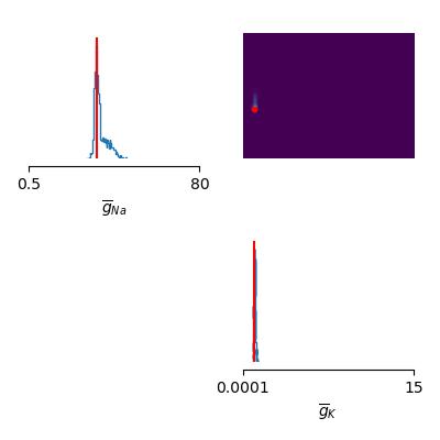
# Plot estimated posterior distribution
samples = posterior.sample((1000,), x=xo, show_progress_bars=False)
labels_params = [r'$\overline{g}_{Na}$', r'$\overline{g}_{K}$']
sbi.analysis.pairplot(samples,
limits=[[.5, 80], [1e-4, 15.]],
ticks=[[.5, 80], [1e-4, 15.]],
figsize=(4, 4),
points=true_params, labels=labels_params,
points_offdiag={'markersize': 6},
points_colors=['r'])
plt.tight_layout()
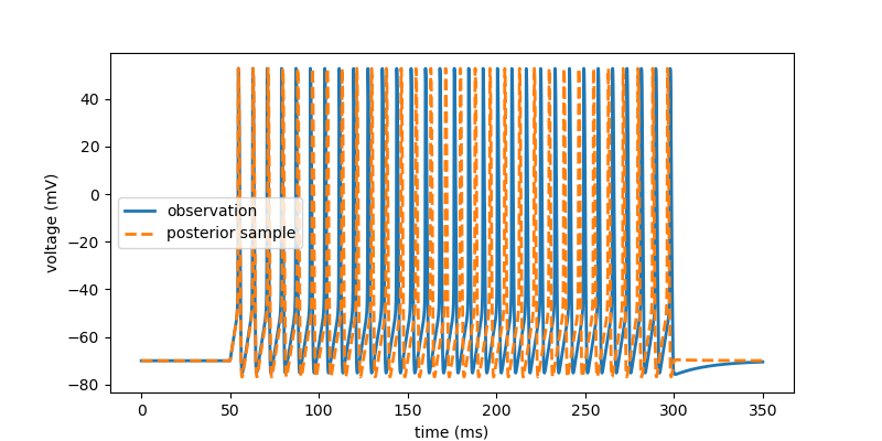
# Draw a single sample from the posterior and convert to numpy for plotting.
posterior_sample = posterior.sample((1,), x=xo,
show_progress_bars=False).numpy()
x = simulate(posterior_sample)
# plot observation and sample
fig, ax = plt.subplots(figsize=(8, 4))
ax.plot(t/ms, v[0, :]/mV, lw=2, label='observation')
ax.plot(t/ms, x['v'][0, :]/mV, '--', lw=2, label='posterior sample')
ax.legend()
ax.set(xlabel='time (ms)', ylabel='voltage (mV)')
plt.show()