Example: exprel_function
Note
You can launch an interactive, editable version of this example without installing any local files using the Binder service (although note that at some times this may be slow or fail to open):
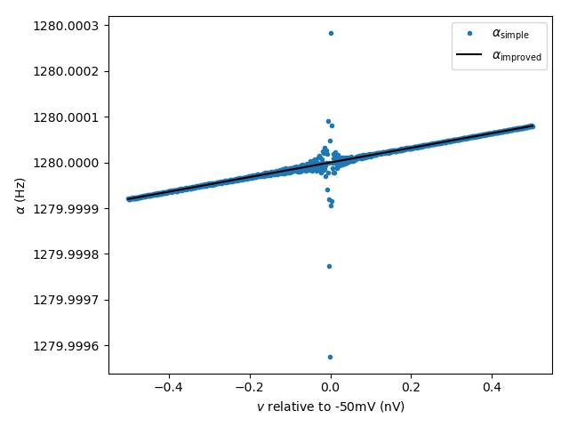
Show the improved numerical accuracy when using the exprel() function in rate equations.
Rate equations for channel opening/closing rates often include a term of the form \(\frac{x}{\exp(x) - 1}\). This term is problematic for two reasons:
It is not defined for \(x = 0\) (where it should equal to \(1\) for continuity);
For values \(x \approx 0\), there is a loss of accuracy.
For better accuracy, and to avoid issues at \(x = 0\), Brian provides the
function exprel(), which is equivalent to \(\frac{\exp(x) - 1}{x}\), but
with better accuracy and the expected result at \(x = 0\). In this example,
we demonstrate the advantage of expressing a typical rate equation from the HH
model with exprel().
from brian2 import *

# Dummy group to evaluate the rate equation at various points
eqs = '''v : volt
         # opening rate from the HH model
         alpha_simple = 0.32*(mV**-1)*(-50*mV-v)/
                        (exp((-50*mV-v)/(4*mV))-1.)/ms : Hz
         alpha_improved = 0.32*(mV**-1)*4*mV/exprel((-50*mV-v)/(4*mV))/ms : Hz'''
neuron = NeuronGroup(1000, eqs)

# Use voltage values around the problematic point
neuron.v = np.linspace(-50 - .5e-6, -50 + .5e-6, len(neuron))*mV

fig, ax = plt.subplots()
ax.plot((neuron.v + 50*mV)/nvolt, neuron.alpha_simple,
         '.', label=r'$\alpha_\mathrm{simple}$')
ax.plot((neuron.v + 50*mV)/nvolt, neuron.alpha_improved,
         'k', label=r'$\alpha_\mathrm{improved}$')
ax.legend()
ax.set(xlabel='$v$ relative to -50mV (nV)', ylabel=r'$\alpha$ (Hz)')
ax.ticklabel_format(useOffset=False)
plt.tight_layout()
plt.show()