Example: lfp

Note

You can launch an interactive, editable version of this example without installing any local files using the Binder service (although note that at some times this may be slow or fail to open):

Hodgkin-Huxley equations (1952)

We calculate the extracellular field potential at various places.

from brian2 import *
defaultclock.dt = 0.01*ms
morpho = Cylinder(x=[0, 10]*cm, diameter=2*238*um, n=1000, type='axon')

El = 10.613* mV
ENa = 115*mV
EK = -12*mV
gl = 0.3*msiemens/cm**2
gNa0 = 120*msiemens/cm**2
gK = 36*msiemens/cm**2

# Typical equations
eqs = '''
# The same equations for the whole neuron, but possibly different parameter values
# distributed transmembrane current
Im = gl * (El-v) + gNa * m**3 * h * (ENa-v) + gK * n**4 * (EK-v) : amp/meter**2
I : amp (point current) # applied current
dm/dt = alpham * (1-m) - betam * m : 1
dn/dt = alphan * (1-n) - betan * n : 1
dh/dt = alphah * (1-h) - betah * h : 1
alpham = (0.1/mV) * 10*mV/exprel((-v+25*mV)/(10*mV))/ms : Hz
betam = 4 * exp(-v/(18*mV))/ms : Hz
alphah = 0.07 * exp(-v/(20*mV))/ms : Hz
betah = 1/(exp((-v+30*mV) / (10*mV)) + 1)/ms : Hz
alphan = (0.01/mV) * 10*mV/exprel((-v+10*mV)/(10*mV))/ms : Hz
betan = 0.125*exp(-v/(80*mV))/ms : Hz
gNa : siemens/meter**2
'''

neuron = SpatialNeuron(morphology=morpho, model=eqs, Cm=1*uF/cm**2,
                       Ri=35.4*ohm*cm, method="exponential_euler")
neuron.v = 0*mV
neuron.h = 1
neuron.m = 0
neuron.n = .5
neuron.I = 0
neuron.gNa = gNa0
neuron[5*cm:10*cm].gNa = 0*siemens/cm**2
M = StateMonitor(neuron, 'v', record=True)

# LFP recorder
Ne = 5 # Number of electrodes
sigma = 0.3*siemens/meter # Resistivity of extracellular field (0.3-0.4 S/m)
lfp = NeuronGroup(Ne, model='''v : volt
                               x : meter
                               y : meter
                               z : meter''')
lfp.x = 7*cm # Off center (to be far from stimulating electrode)
lfp.y = [1*mm, 2*mm, 4*mm, 8*mm, 16*mm]
S = Synapses(neuron, lfp, model='''w : ohm*meter**2 (constant) # Weight in the LFP calculation
                                   v_post = w*(Ic_pre-Im_pre) : volt (summed)''')
S.summed_updaters['v_post'].when = 'after_groups'  # otherwise Ic has not yet been updated for the current time step.
S.connect()
S.w = 'area_pre/(4*pi*sigma)/((x_pre-x_post)**2+(y_pre-y_post)**2+(z_pre-z_post)**2)**.5'

Mlfp = StateMonitor(lfp, 'v', record=True)

run(50*ms, report='text')
neuron.I[0] = 1*uA  # current injection at one end
run(3*ms)
neuron.I = 0*amp
run(100*ms, report='text')

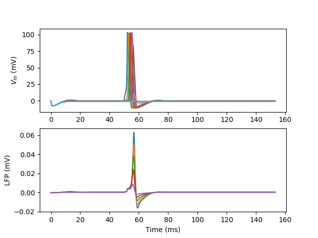
subplot(211)
for i in range(10):
    plot(M.t/ms, M.v[i*100]/mV)
ylabel('$V_m$ (mV)')
subplot(212)
for i in range(5):
    plot(M.t/ms, Mlfp.v[i]/mV)
ylabel('LFP (mV)')
xlabel('Time (ms)')
show()