Example: standalone_multiplerun
Note
You can launch an interactive, editable version of this example without installing any local files using the Binder service (although note that at some times this may be slow or fail to open):
This example shows how to run several, independent simulations in standalone mode.
Given that this example only involves a single neuron, an alternative – and arguably more elegant – solution
would be to run the simulations in a single NeuronGroup, where each neuron receives input with a different rate.
The example is a standalone equivalent of the one presented in /tutorials/3-intro-to-brian-simulations.
import numpy as np
import matplotlib.pyplot as plt
import brian2 as b2
from time import time
b2.set_device('cpp_standalone', build_on_run=False)
if __name__ == "__main__":
start_time = time()
num_inputs = 100
input_rate = 10 * b2.Hz
weight = 0.1
net = b2.Network()
P = b2.PoissonGroup(num_inputs, rates=input_rate)
eqs = """
dv/dt = -v/tau : 1
tau : second (constant)
"""
G = b2.NeuronGroup(1, eqs, threshold='v>1', reset='v=0', method='euler')
S = b2.Synapses(P, G, on_pre='v += weight')
S.connect()
M = b2.SpikeMonitor(G)
net.add([P, G, S, M])
net.run(1000 * b2.ms)
b2.device.build(run=False) # compile the code, but don't run it yet
npoints = 15
tau_range = np.linspace(1, 15, npoints) * b2.ms
output_rates = np.zeros(npoints)
for ii in range(npoints):
tau_i = tau_range[ii]
b2.device.run(run_args={G.tau: tau_i})
output_rates[ii] = M.num_spikes / b2.second
print(f"Done in {time() - start_time}")
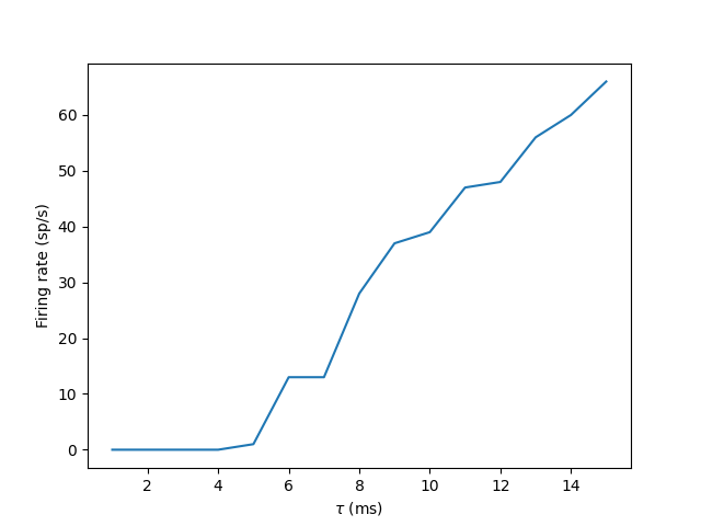
plt.plot(tau_range/b2.ms, output_rates)
plt.xlabel(r"$\tau$ (ms)")
plt.ylabel("Firing rate (sp/s)")
plt.show()