Example: example_3_io_synapse
Note
You can launch an interactive, editable version of this example without installing any local files using the Binder service (although note that at some times this may be slow or fail to open):
Modeling neuron-glia interactions with the Brian 2 simulator Marcel Stimberg, Dan F. M. Goodman, Romain Brette, Maurizio De Pittà bioRxiv 198366; doi: https://doi.org/10.1101/198366
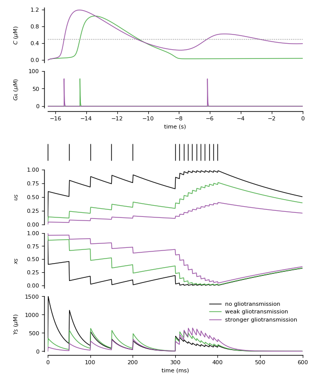
Figure 3: Modeling of modulation of synaptic release by gliotransmission.
Three synapses: the first one without astrocyte, the remaining two respectively with open-loop and close-loop gliotransmission (see De Pitta’ et al., 2011, 2016)
from brian2 import *

import plot_utils as pu

set_device('cpp_standalone', directory=None)  # Use fast "C++ standalone mode"

################################################################################
# Model parameters
################################################################################
### General parameters
transient = 16.5*second
duration = transient + 600*ms   # Total simulation time
sim_dt = 1*ms                   # Integrator/sampling step

### Synapse parameters
rho_c = 0.005                   # Synaptic vesicle-to-extracellular space volume ratio
Y_T = 500*mmolar                # Total vesicular neurotransmitter concentration
Omega_c = 40/second             # Neurotransmitter clearance rate
U_0__star = 0.6                 # Resting synaptic release probability
Omega_f = 3.33/second           # Synaptic facilitation rate
Omega_d = 2.0/second            # Synaptic depression rate
# --- Presynaptic receptors
O_G = 1.5/umolar/second         # Agonist binding (activating) rate
Omega_G = 0.5/(60*second)       # Agonist release (deactivating) rate

### Astrocyte parameters
# ---  Calcium fluxes
O_P = 0.9*umolar/second         # Maximal Ca^2+ uptake rate by SERCAs
K_P = 0.05 * umolar             # Ca2+ affinity of SERCAs
C_T = 2*umolar                  # Total cell free Ca^2+ content
rho_A = 0.18                    # ER-to-cytoplasm volume ratio
Omega_C = 6/second              # Maximal rate of Ca^2+ release by IP_3Rs
Omega_L = 0.1/second            # Maximal rate of Ca^2+ leak from the ER
# --- IP_3R kinectics
d_1 = 0.13*umolar               # IP_3 binding affinity
d_2 = 1.05*umolar               # Ca^2+ inactivation dissociation constant
O_2 = 0.2/umolar/second         # IP_3R binding rate for Ca^2+ inhibition
d_3 = 0.9434*umolar             # IP_3 dissociation constant
d_5 = 0.08*umolar               # Ca^2+ activation dissociation constant
# --- IP_3 production
O_delta = 0.6*umolar/second     # Maximal rate of IP_3 production by PLCdelta
kappa_delta = 1.5* umolar       # Inhibition constant of PLC_delta by IP_3
K_delta = 0.1*umolar            # Ca^2+ affinity of PLCdelta
# --- IP_3 degradation
Omega_5P = 0.05/second          # Maximal rate of IP_3 degradation by IP-5P
K_D = 0.7*umolar                # Ca^2+ affinity of IP3-3K
K_3K = 1.0*umolar               # IP_3 affinity of IP_3-3K
O_3K = 4.5*umolar/second        # Maximal rate of IP_3 degradation by IP_3-3K
# --- IP_3 diffusion
F_ex = 2.0*umolar/second        # Maximal exogenous IP3 flow
I_Theta = 0.3*umolar            # Threshold gradient for IP_3 diffusion
omega_I = 0.05*umolar           # Scaling factor of diffusion
# --- Gliotransmitter release and time course
C_Theta = 0.5*umolar            # Ca^2+ threshold for exocytosis
Omega_A = 0.6/second            # Gliotransmitter recycling rate
U_A = 0.6                       # Gliotransmitter release probability
G_T = 200*mmolar                # Total vesicular gliotransmitter concentration
rho_e = 6.5e-4                  # Astrocytic vesicle-to-extracellular volume ratio
Omega_e = 60/second             # Gliotransmitter clearance rate
alpha = 0.0                     # Gliotransmission nature

################################################################################
# Model definition
################################################################################
defaultclock.dt = sim_dt  # Set the integration time

### "Neurons"
# We are only interested in the activity of the synapse, so we replace the
# neurons by trivial "dummy" groups
spikes = [0, 50, 100, 150, 200,
          300, 310, 320, 330, 340, 350, 360, 370, 380, 390, 400]*ms
spikes += transient  # allow for some initial transient
source_neurons = SpikeGeneratorGroup(1, np.zeros(len(spikes)), spikes)
target_neurons = NeuronGroup(1, '')

### Synapses
# Note that the synapse does not actually have any effect on the post-synaptic
# target
# Also note that for easier plotting we do not use the "event-driven" flag here,
# even though the value of u_S and x_S only needs to be updated on the arrival
# of a spike
synapses_eqs = '''
# Neurotransmitter
dY_S/dt = -Omega_c * Y_S        : mmolar (clock-driven)
# Fraction of activated presynaptic receptors
dGamma_S/dt = O_G * G_A * (1 - Gamma_S) -
              Omega_G * Gamma_S : 1 (clock-driven)
# Usage of releasable neurotransmitter per single action potential:
du_S/dt = -Omega_f * u_S        : 1 (clock-driven)
# Fraction of synaptic neurotransmitter resources available:
dx_S/dt = Omega_d *(1 - x_S)    : 1 (clock-driven)
# released synaptic neurotransmitter resources:
r_S                             : 1
# gliotransmitter concentration in the extracellular space:
G_A                             : mmolar
'''
synapses_action = '''
U_0 = (1 - Gamma_S) * U_0__star + alpha * Gamma_S
u_S += U_0 * (1 - u_S)
r_S = u_S * x_S
x_S -= r_S
Y_S += rho_c * Y_T * r_S
'''
synapses = Synapses(source_neurons, target_neurons,
                    model=synapses_eqs, on_pre=synapses_action,
                    method='exact')
# We create three synapses, only the second and third ones are modulated by astrocytes
synapses.connect(True, n=3)

### Astrocytes
# The astrocyte emits gliotransmitter when its Ca^2+ concentration crosses
# a threshold
astro_eqs = '''
# IP_3 dynamics:
dI/dt = J_delta - J_3K - J_5P + J_ex                             : mmolar
J_delta = O_delta/(1 + I/kappa_delta) * C**2/(C**2 + K_delta**2) : mmolar/second
J_3K = O_3K * C**4/(C**4 + K_D**4) * I/(I + K_3K)                : mmolar/second
J_5P = Omega_5P*I                                                : mmolar/second
# Exogenous stimulation
delta_I_bias = I - I_bias          : mmolar
J_ex = -F_ex/2*(1 + tanh((abs(delta_I_bias) - I_Theta)/omega_I)) *
                sign(delta_I_bias) : mmolar/second
I_bias                             : mmolar (constant)

# Ca^2+-induced Ca^2+ release:
dC/dt = (Omega_C * m_inf**3 * h**3 + Omega_L) * (C_T - (1 + rho_A)*C) -
        O_P * C**2/(C**2 + K_P**2) : mmolar
dh/dt = (h_inf - h)/tau_h : 1  # IP3R de-inactivation probability
m_inf = I/(I + d_1) * C/(C + d_5)  : 1
h_inf = Q_2/(Q_2 + C)              : 1
tau_h = 1/(O_2 * (Q_2 + C))        : second
Q_2 = d_2 * (I + d_1)/(I + d_3)    : mmolar
# Fraction of gliotransmitter resources available:
dx_A/dt = Omega_A * (1 - x_A)      : 1
# gliotransmitter concentration in the extracellular space:
dG_A/dt = -Omega_e*G_A             : mmolar
'''
glio_release = '''
G_A += rho_e * G_T * U_A * x_A
x_A -= U_A *  x_A
'''
# The following formulation makes sure that a "spike" is only triggered at the
# first threshold crossing -- the astrocyte is considered "refractory" (i.e.,
# not allowed to trigger another event) as long as the Ca2+ concentration
# remains above threshold
# The gliotransmitter release happens when the threshold is crossed, in Brian
# terms it can therefore be considered a "reset"
astrocyte = NeuronGroup(2, astro_eqs,
                        threshold='C>C_Theta',
                        refractory='C>C_Theta',
                        reset=glio_release,
                        method='rk4')
# Different length of stimulation
astrocyte.x_A = 1.0
astrocyte.h = 0.9
astrocyte.I = 0.4*umolar
astrocyte.I_bias = np.asarray([0.8, 1.25])*umolar

# Connection between astrocytes and the second synapse. Note that in this
# special case, where the synapse is only influenced by the gliotransmitter from
# a single astrocyte, the '(linked)' variable mechanism could be used instead.
# The mechanism used below is more general and can add the contribution of
# several astrocytes
ecs_astro_to_syn = Synapses(astrocyte, synapses,
                            'G_A_post = G_A_pre : mmolar (summed)')
# Connect second and third synapse to a different astrocyte
ecs_astro_to_syn.connect(j='i+1')

################################################################################
# Monitors
################################################################################
# Note that we cannot use "record=True" for synapses in C++ standalone mode --
# the StateMonitor needs to know the number of elements to record from during
# its initialization, but in C++ standalone mode, no synapses have been created
# yet. We therefore explicitly state to record from the three synapses.
syn_mon = StateMonitor(synapses, variables=['u_S', 'x_S', 'r_S', 'Y_S'],
                       record=[0, 1, 2])
ast_mon = StateMonitor(astrocyte, variables=['C', 'G_A'], record=True)

################################################################################
# Simulation run
################################################################################
run(duration, report='text')

################################################################################
# Analysis and plotting
################################################################################
from matplotlib import cycler
plt.style.use('figures.mplstyle')

fig, ax = plt.subplots(nrows=7, ncols=1, figsize=(6.26894, 6.26894 * 1.2),
                       gridspec_kw={'height_ratios': [3, 2, 1, 1, 3, 3, 3],
                                    'top': 0.98, 'bottom': 0.08,
                                    'left': 0.15, 'right': 0.95})

## Ca^2+ traces of the two astrocytes
ax[0].plot((ast_mon.t-transient)/second, ast_mon.C[0]/umolar, '-', color='C2')
ax[0].plot((ast_mon.t-transient)/second, ast_mon.C[1]/umolar, '-', color='C3')
## Add threshold for gliotransmitter release
ax[0].plot(np.asarray([-transient/second, 0.0]),
           np.asarray([C_Theta, C_Theta])/umolar, ':', color='gray')
ax[0].set(xlim=[-transient/second, 0.0], yticks=[0., 0.4, 0.8, 1.2],
          ylabel=r'$C$ ($\mu$M)')
pu.adjust_spines(ax[0], ['left'])

## Gliotransmitter concentration in the extracellular space
ax[1].plot((ast_mon.t-transient)/second, ast_mon.G_A[0]/umolar, '-', color='C2')
ax[1].plot((ast_mon.t-transient)/second, ast_mon.G_A[1]/umolar, '-', color='C3')
ax[1].set(yticks=[0., 50., 100.], xlim=[-transient/second, 0.0],
          xlabel='time (s)', ylabel=r'$G_A$ ($\mu$M)')
pu.adjust_spines(ax[1], ['left', 'bottom'])

## Turn off one axis to display x-labeling of ax[1] correctly
ax[2].axis('off')

## Synaptic stimulation
ax[3].vlines((spikes-transient)/ms, 0, 1, clip_on=False)
ax[3].set(xlim=(0, (duration-transient)/ms))
ax[3].axis('off')

## Synaptic variables
# Use a custom cycle that uses black as the first color
prop_cycle = cycler(color='k').concat(matplotlib.rcParams['axes.prop_cycle'][2:])
ax[4].set(xlim=(0, (duration-transient)/ms), ylim=[0., 1.],
          yticks=np.arange(0, 1.1, .25), ylabel='$u_S$',
          prop_cycle=prop_cycle)
ax[4].plot((syn_mon.t-transient)/ms, syn_mon.u_S.T)
pu.adjust_spines(ax[4], ['left'])

ax[5].set(xlim=(0, (duration-transient)/ms), ylim=[-0.05, 1.],
          yticks=np.arange(0, 1.1, .25), ylabel='$x_S$',
          prop_cycle=prop_cycle)
ax[5].plot((syn_mon.t-transient)/ms, syn_mon.x_S.T)
pu.adjust_spines(ax[5], ['left'])

ax[6].set(xlim=(0, (duration-transient)/ms), ylim=(-5., 1500),
          xticks=np.arange(0, (duration-transient)/ms, 100), xlabel='time (ms)',
          yticks=[0, 500, 1000, 1500], ylabel=r'$Y_S$ ($\mu$M)',
          prop_cycle=prop_cycle)
ax[6].plot((syn_mon.t-transient)/ms, syn_mon.Y_S.T/umolar)
ax[6].legend(['no gliotransmission',
              'weak gliotransmission',
              'stronger gliotransmission'], loc='upper right')
pu.adjust_spines(ax[6], ['left', 'bottom'])

pu.adjust_ylabels(ax, x_offset=-0.11)

plt.show()