Example: STDP_standalone
Note
You can launch an interactive, editable version of this example without installing any local files using the Binder service (although note that at some times this may be slow or fail to open):
Spike-timing dependent plasticity. Adapted from Song, Miller and Abbott (2000) and Song and Abbott (2001).
This example is modified from synapses_STDP.py and writes a standalone
C++ project in the directory STDP_standalone.
from brian2 import *
set_device('cpp_standalone', directory='STDP_standalone')
N = 1000
taum = 10*ms
taupre = 20*ms
taupost = taupre
Ee = 0*mV
vt = -54*mV
vr = -60*mV
El = -74*mV
taue = 5*ms
F = 15*Hz
gmax = .01
dApre = .01
dApost = -dApre * taupre / taupost * 1.05
dApost *= gmax
dApre *= gmax
eqs_neurons = '''
dv/dt = (ge * (Ee-v) + El - v) / taum : volt
dge/dt = -ge / taue : 1
'''
input = PoissonGroup(N, rates=F)
neurons = NeuronGroup(1, eqs_neurons, threshold='v>vt', reset='v = vr',
method='euler')
S = Synapses(input, neurons,
'''w : 1
dApre/dt = -Apre / taupre : 1 (event-driven)
dApost/dt = -Apost / taupost : 1 (event-driven)''',
on_pre='''ge += w
Apre += dApre
w = clip(w + Apost, 0, gmax)''',
on_post='''Apost += dApost
w = clip(w + Apre, 0, gmax)''',
)
S.connect()
S.w = 'rand() * gmax'
mon = StateMonitor(S, 'w', record=[0, 1])
s_mon = SpikeMonitor(input)
run(100*second, report='text')
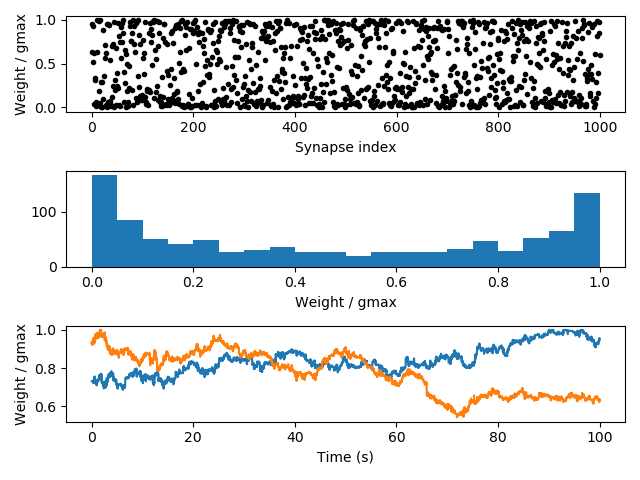
subplot(311)
plot(S.w / gmax, '.k')
ylabel('Weight / gmax')
xlabel('Synapse index')
subplot(312)
hist(S.w / gmax, 20)
xlabel('Weight / gmax')
subplot(313)
plot(mon.t/second, mon.w.T/gmax)
xlabel('Time (s)')
ylabel('Weight / gmax')
tight_layout()
show()