Example: Fig3CF
Note
You can launch an interactive, editable version of this example without installing any local files using the Binder service (although note that at some times this may be slow or fail to open):
Brette R (2013). Sharpness of spike initiation in neurons explained by compartmentalization. PLoS Comp Biol, doi: 10.1371/journal.pcbi.1003338.
Fig. 3C-F. Kink with Nav1.6 and Nav1.2
from brian2 import *
from params import *
defaultclock.dt = 0.01*ms
# Morphology
morpho = Soma(50*um) # chosen for a target Rm
morpho.axon = Cylinder(diameter=1*um, length=300*um, n=300)
location16 = 40*um # where Nav1.6 channels are placed
location12 = 15*um # where Nav1.2 channels are placed
va2 = va + 15*mV # depolarized Nav1.2
# Channels
duration = 100*ms
eqs='''
Im = gL * (EL - v) + gNa*m*(ENa - v) + gNa2*m2*(ENa - v) : amp/meter**2
dm/dt = (minf - m) / taum : 1 # simplified Na channel
minf = 1 / (1 + exp((va - v) / ka)) : 1
dm2/dt = (minf2 - m2) / taum : 1 # simplified Na channel, Nav1.2
minf2 = 1/(1 + exp((va2 - v) / ka)) : 1
gNa : siemens/meter**2
gNa2 : siemens/meter**2 # Nav1.2
Iin : amp (point current)
'''
neuron = SpatialNeuron(morphology=morpho, model=eqs, Cm=Cm, Ri=Ri,
method="exponential_euler")
compartment16 = morpho.axon[location16]
compartment12 = morpho.axon[location12]
neuron.v = EL
neuron.gNa[compartment16] = gNa_0/neuron.area[compartment16]
neuron.gNa2[compartment12] = 20*gNa_0/neuron.area[compartment12]
# Monitors
M = StateMonitor(neuron, ['v', 'm', 'm2'], record=True)
run(20*ms, report='text')
neuron.Iin[0] = gL * 20*mV * neuron.area[0]
run(80*ms, report='text')
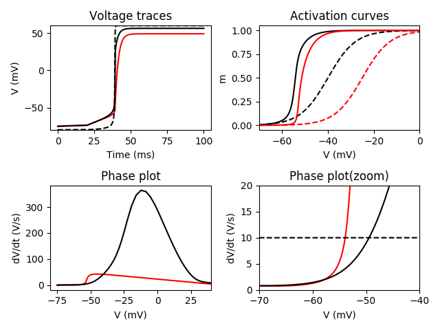
subplot(221)
plot(M.t/ms, M[0].v/mV, 'r')
plot(M.t/ms, M[compartment16].v/mV, 'k')
plot(M.t/ms, M[compartment16].m*(80+60)-80, 'k--') # open channels
ylim(-80, 60)
xlabel('Time (ms)')
ylabel('V (mV)')
title('Voltage traces')
subplot(222)
plot(M[0].v/mV, M[compartment16].m, 'k')
plot(M[0].v/mV, 1 / (1 + exp((va - M[0].v) / ka)), 'k--')
plot(M[0].v/mV, M[compartment12].m2, 'r')
plot(M[0].v/mV, 1 / (1 + exp((va2 - M[0].v) / ka)), 'r--')
xlim(-70, 0)
xlabel('V (mV)')
ylabel('m')
title('Activation curves')
subplot(223)
dm = diff(M[0].v) / defaultclock.dt
dm40 = diff(M[compartment16].v) / defaultclock.dt
plot((M[0].v/mV)[1:], dm/(volt/second), 'r')
plot((M[compartment16].v/mV)[1:], dm40/(volt/second), 'k')
xlim(-80, 40)
xlabel('V (mV)')
ylabel('dV/dt (V/s)')
title('Phase plot')
subplot(224)
plot((M[0].v/mV)[1:], dm/(volt/second), 'r')
plot((M[compartment16].v/mV)[1:], dm40/(volt/second), 'k')
plot((M[0].v/mV)[1:], 10 + 0*dm/(volt/second), 'k--')
xlim(-70, -40)
ylim(0, 20)
xlabel('V (mV)')
ylabel('dV/dt (V/s)')
title('Phase plot(zoom)')
tight_layout()
show()