Example: Ornstein_Uhlenbeck
Note
You can launch an interactive, editable version of this example without installing any local files using the Binder service (although note that at some times this may be slow or fail to open):
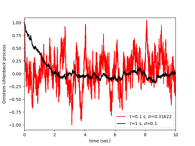
Ornstein-Uhlenbeck process
Figure 2: Two realizations of the Ornstein-Uhlenbeck process for parameters τ=1.0 and σ=0.1 (black curve), and for τ=0.1 and σ=0.31622 (red curve). In both cases the noise intensity is σ^2*τ=0.01 . The red curve represents a noise that more closely mimics Gaussian white noise. Both realizations begin here at x(0)=1.0 , after which the mean decays exponentially to zero with time constant τ.
Andre Longtin (2010) Stochastic dynamical systems. Scholarpedia, 5(4):1619.
Sebastian Schmitt, 2022
import matplotlib.pyplot as plt
import numpy as np

from brian2 import run
from brian2 import NeuronGroup, StateMonitor
from brian2 import second, ms

N = NeuronGroup(
    2,
    """
    tau : second
    sigma : 1
    dy/dt = -y/tau + sqrt(2*sigma**2/tau)*xi : 1
    """,
    method="euler"
)

N.tau = np.array([1, 0.1]) * second
N.sigma = np.array([0.1, 0.31622])
N.y = 1

M = StateMonitor(N, "y", record=True)

run(10 * second)

plt.plot(M.t / second, M.y[1], color="red", label=r"$\tau$=0.1 s, $\sigma$=0.31622")
plt.plot(M.t / second, M.y[0], color="k", label=r"$\tau$=1 s, $\sigma$=0.1")

plt.xlim(0, 10)
plt.ylim(-1.1, 1.1)

plt.xlabel("time (sec)")
plt.ylabel("Ornstein-Uhlenbeck process")

plt.legend()

plt.show()