Example: infinite_cable
Note
You can launch an interactive, editable version of this example without installing any local files using the Binder service (although note that at some times this may be slow or fail to open):
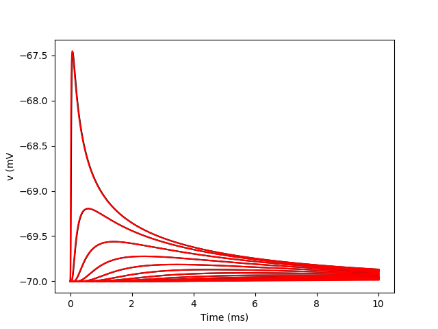
An (almost) infinite cable with pulse injection in the middle.
from brian2 import *

defaultclock.dt = 0.001*ms

# Morphology
diameter = 1*um
Cm = 1*uF/cm**2
Ri = 100*ohm*cm
N = 500
morpho = Cylinder(diameter=diameter, length=3*mm, n=N)

# Passive channels
gL = 1e-4*siemens/cm**2
EL = -70*mV
eqs = '''
Im = gL * (EL-v) : amp/meter**2
I : amp (point current)
'''

neuron = SpatialNeuron(morphology=morpho, model=eqs, Cm=Cm, Ri=Ri,
                       method = 'exponential_euler')
neuron.v = EL

taum = Cm  /gL  # membrane time constant
print("Time constant: %s" % taum)
la = neuron.space_constant[0]
print("Characteristic length: %s" % la)

# Monitors
mon = StateMonitor(neuron, 'v', record=range(0, N//2, 20))

neuron.I[len(neuron) // 2] = 1*nA  # injecting in the middle
run(0.02*ms)
neuron.I = 0*amp
run(10*ms, report='text')

t = mon.t
plot(t/ms, mon.v.T/mV, 'k')
# Theory (incorrect near cable ends)
for i in range(0, len(neuron)//2, 20):
    x = (len(neuron)/2 - i) * morpho.length[0]
    theory = (1/(la*Cm*pi*diameter) * sqrt(taum / (4*pi*(t + defaultclock.dt))) *
              exp(-(t+defaultclock.dt)/taum -
                  taum / (4*(t+defaultclock.dt))*(x/la)**2))
    theory = EL + theory * 1*nA * 0.02*ms
    plot(t/ms, theory/mV, 'r')
xlabel('Time (ms)')
ylabel('v (mV')
show()