Example: Hindmarsh_Rose_1984
Note
You can launch an interactive, editable version of this example without installing any local files using the Binder service (although note that at some times this may be slow or fail to open):
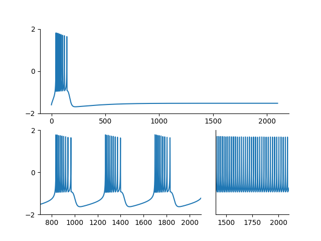
Burst generation in the Hinsmarsh-Rose model. Reproduces Figure 6 of:
Hindmarsh, J. L., and R. M. Rose. “A Model of Neuronal Bursting Using Three Coupled First Order Differential Equations.” Proceedings of the Royal Society of London. Series B, Biological Sciences 221, no. 1222 (1984): 87–102.
from brian2 import *

# In the original model, time is measured in arbitrary time units
time_unit = 1*ms
defaultclock.dt = time_unit/10

x_1 = -1.6  # leftmost equilibrium point of the model without adaptation
a = 1; b = 3; c = 1; d = 5
r = 0.001; s = 4
eqs = '''
dx/dt = (y - a*x**3 + b*x**2 + I - z)/time_unit : 1
dy/dt = (c - d*x**2 - y)/time_unit : 1
dz/dt = r*(s*(x - x_1) - z)/time_unit : 1
I : 1 (constant)
'''

# We run the model with three different currents
neuron = NeuronGroup(3, eqs, method='rk4')

# Set all variables to their equilibrium point
neuron.x = x_1
neuron.y = 'c - d*x**2'
neuron.z = 'r*(s*(x - x_1))'

# Set the constant current input
neuron.I = [0.4, 2, 4]

# Record the "membrane potential"
mon = StateMonitor(neuron, 'x', record=True)

run(2100*time_unit)

ax_top = plt.subplot2grid((2, 3), (0, 0), colspan=3)
ax_bottom_l = plt.subplot2grid((2, 3), (1, 0), colspan=2)
ax_bottom_r = plt.subplot2grid((2, 3), (1, 2))
for ax in [ax_top, ax_bottom_l, ax_bottom_r]:
    ax.spines['top'].set_visible(False)
    ax.spines['right'].set_visible(False)
    ax.set(ylim=(-2, 2), yticks=[-2, 0, 2])

ax_top.plot(mon.t/time_unit, mon.x[0])

ax_bottom_l.plot(mon.t/time_unit, mon.x[1])
ax_bottom_l.set_xlim(700, 2100)

ax_bottom_r.plot(mon.t/time_unit, mon.x[2])
ax_bottom_r.set_xlim(1400, 2100)
ax_bottom_r.set_yticks([])

plt.show()