Example: Brette_Gerstner_2005
Note
You can launch an interactive, editable version of this example without installing any local files using the Binder service (although note that at some times this may be slow or fail to open):
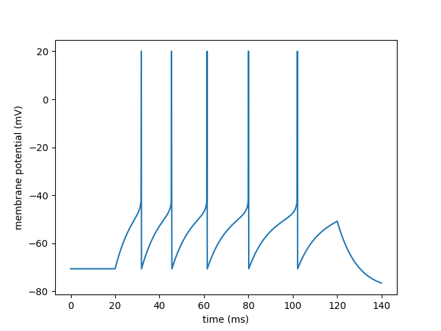
Adaptive exponential integrate-and-fire model.
http://www.scholarpedia.org/article/Adaptive_exponential_integrate-and-fire_model
Introduced in Brette R. and Gerstner W. (2005), Adaptive Exponential Integrate-and-Fire Model as an Effective Description of Neuronal Activity, J. Neurophysiol. 94: 3637 - 3642.
from brian2 import *

# Parameters
C = 281 * pF
gL = 30 * nS
taum = C / gL
EL = -70.6 * mV
VT = -50.4 * mV
DeltaT = 2 * mV
Vcut = VT + 5 * DeltaT

# Pick an electrophysiological behaviour
tauw, a, b, Vr = 144*ms, 4*nS, 0.0805*nA, -70.6*mV # Regular spiking (as in the paper)
#tauw,a,b,Vr=20*ms,4*nS,0.5*nA,VT+5*mV # Bursting
#tauw,a,b,Vr=144*ms,2*C/(144*ms),0*nA,-70.6*mV # Fast spiking

eqs = """
dvm/dt = (gL*(EL - vm) + gL*DeltaT*exp((vm - VT)/DeltaT) + I - w)/C : volt
dw/dt = (a*(vm - EL) - w)/tauw : amp
I : amp
"""

neuron = NeuronGroup(1, model=eqs, threshold='vm>Vcut',
                     reset="vm=Vr; w+=b", method='euler')
neuron.vm = EL
trace = StateMonitor(neuron, 'vm', record=0)
spikes = SpikeMonitor(neuron)

run(20 * ms)
neuron.I = 1*nA
run(100 * ms)
neuron.I = 0*nA
run(20 * ms)

# We draw nicer spikes
vm = trace[0].vm[:]
for t in spikes.t:
    i = int(t / defaultclock.dt)
    vm[i] = 20*mV

plot(trace.t / ms, vm / mV)
xlabel('time (ms)')
ylabel('membrane potential (mV)')
show()