Example: bipolar_with_inputs2
Note
You can launch an interactive, editable version of this example without installing any local files using the Binder service (although note that at some times this may be slow or fail to open):
A pseudo MSO neuron, with two dendrites (fake geometry). There are synaptic inputs.
Second method.
from brian2 import *
# Morphology
morpho = Soma(30*um)
morpho.L = Cylinder(diameter=1*um, length=100*um, n=50)
morpho.R = Cylinder(diameter=1*um, length=100*um, n=50)
# Passive channels
gL = 1e-4*siemens/cm**2
EL = -70*mV
Es = 0*mV
taus = 1*ms
eqs='''
Im = gL*(EL-v) : amp/meter**2
Is = gs*(Es-v) : amp (point current)
dgs/dt = -gs/taus : siemens
'''
neuron = SpatialNeuron(morphology=morpho, model=eqs,
Cm=1*uF/cm**2, Ri=100*ohm*cm, method='exponential_euler')
neuron.v = EL
# Regular inputs
stimulation = NeuronGroup(2, 'dx/dt = 300*Hz : 1', threshold='x>1', reset='x=0',
method='euler')
stimulation.x = [0, 0.5] # Asynchronous
# Synapses
w = 20*nS
S = Synapses(stimulation, neuron, on_pre='gs += w')
S.connect(i=0, j=morpho.L[99.9*um])
S.connect(i=1, j=morpho.R[99.9*um])
# Monitors
mon_soma = StateMonitor(neuron, 'v', record=[0])
mon_L = StateMonitor(neuron.L, 'v', record=True)
mon_R = StateMonitor(neuron, 'v', record=morpho.R[99.9*um])
run(50*ms, report='text')
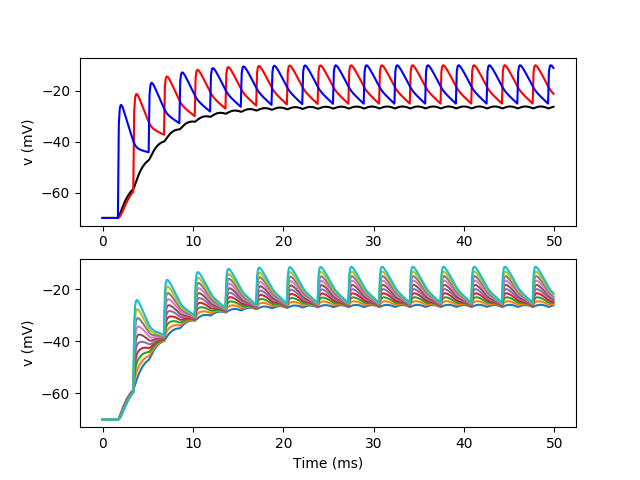
subplot(211)
plot(mon_L.t/ms, mon_soma[0].v/mV, 'k')
plot(mon_L.t/ms, mon_L[morpho.L[99.9*um]].v/mV, 'r')
plot(mon_L.t/ms, mon_R[morpho.R[99.9*um]].v/mV, 'b')
ylabel('v (mV)')
subplot(212)
for i in [0, 5, 10, 15, 20, 25, 30, 35, 40, 45]:
plot(mon_L.t/ms, mon_L.v[i, :]/mV)
xlabel('Time (ms)')
ylabel('v (mV)')
show()