Example: Naud_et_al_2008_adex_firing_patterns
Note
You can launch an interactive, editable version of this example without installing any local files using the Binder service (although note that at some times this may be slow or fail to open):
Firing patterns in the adaptive exponential integrate-and-fire model
Naud R et al. (2008): Firing patterns in the adaptive exponential integrate-and-fire model. Biol Cybern. 2008; 99(4): 335–347. doi:10.1007/s00422-008-0264-7
Parameters adapted by P. Müller to match figures, cf. http://www.kip.uni-heidelberg.de/Veroeffentlichungen/details.php?id=3445.
Sebastian Schmitt, Sebastian Billaudelle, 2022
from brian2 import *
import matplotlib.pyplot as plt
def sim(ax_vm, ax_w, ax_vm_w, parameters):
"""
simulate with parameters and plot to axes
"""
# taken from Touboul_Brette_2008
eqs = """
dvm/dt = (g_l*(e_l - vm) + g_l*d_t*exp((vm-v_t)/d_t) + i_stim - w)/c_m : volt
dw/dt = (a*(vm - e_l) - w)/tau_w : amp
"""
neuron = NeuronGroup(
1,
model=eqs,
threshold="vm > 0*mV",
reset="vm = v_r; w += b",
method="euler",
namespace=parameters,
)
neuron.vm = parameters["e_l"]
neuron.w = 0
states = StateMonitor(neuron, ["vm", "w"], record=True, when="thresholds")
defaultclock.dt = 0.1 * ms
run(0.6 * second)
# clip membrane voltages to threshold (0 mV)
vms = np.clip(states[0].vm / mV, a_min=None, a_max=0)
ax_vm.plot(states[0].t / ms, vms)
ax_w.plot(states[0].t / ms, states[0].w / nA)
ax_vm_w.plot(vms, states[0].w / nA)
ax_w.sharex(ax_vm)
ax_vm.tick_params(labelbottom=False)
ax_vm.set_ylabel("V [mV]")
ax_w.set_xlabel("t [ms]")
ax_w.set_ylabel("w [nA]")
ax_vm_w.set_xlabel("V [mV]")
ax_vm_w.set_ylabel("w [nA]")
ax_vm_w.yaxis.tick_right()
ax_vm_w.yaxis.set_label_position("right")
patterns = {
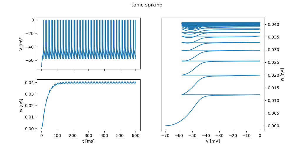
"tonic spiking": {
"c_m": 200 * pF,
"g_l": 10 * nS,
"e_l": -70.0 * mV,
"v_t": -50.0 * mV,
"d_t": 2.0 * mV,
"a": 2.0 * nS,
"tau_w": 30.0 * ms,
"b": 0.0 * pA,
"v_r": -58.0 * mV,
"i_stim": 500 * pA,
},
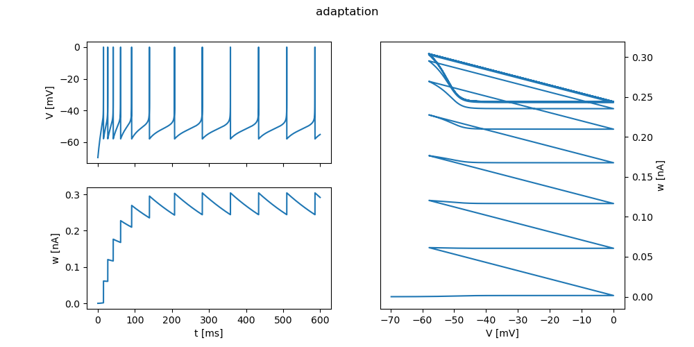
"adaptation": {
"c_m": 200 * pF,
"g_l": 12 * nS,
"e_l": -70.0 * mV,
"v_t": -50.0 * mV,
"d_t": 2.0 * mV,
"a": 2.0 * nS,
"tau_w": 300.0 * ms,
"b": 60.0 * pA,
"v_r": -58.0 * mV,
"i_stim": 500 * pA,
},
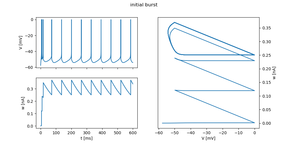
"initial burst": {
"c_m": 130 * pF,
"g_l": 18 * nS,
"e_l": -58.0 * mV,
"v_t": -50.0 * mV,
"d_t": 2.0 * mV,
"a": 4.0 * nS,
"tau_w": 150.0 * ms,
"b": 120.0 * pA,
"v_r": -50.0 * mV,
"i_stim": 400 * pA,
},
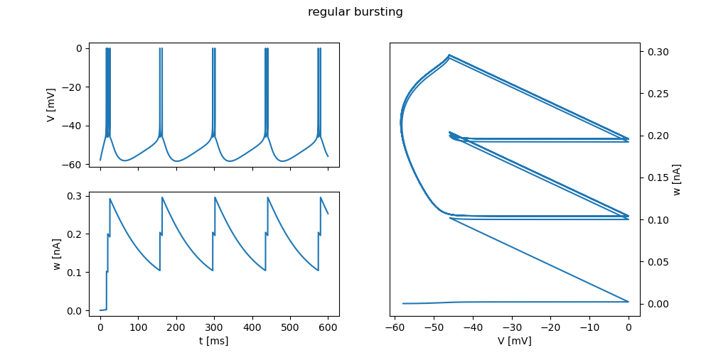
"regular bursting": {
"c_m": 200 * pF,
"g_l": 10 * nS,
"e_l": -58.0 * mV,
"v_t": -50.0 * mV,
"d_t": 2.0 * mV,
"a": 2.0 * nS,
"tau_w": 120.0 * ms,
"b": 100.0 * pA,
"v_r": -46.0 * mV,
"i_stim": 210 * pA,
},
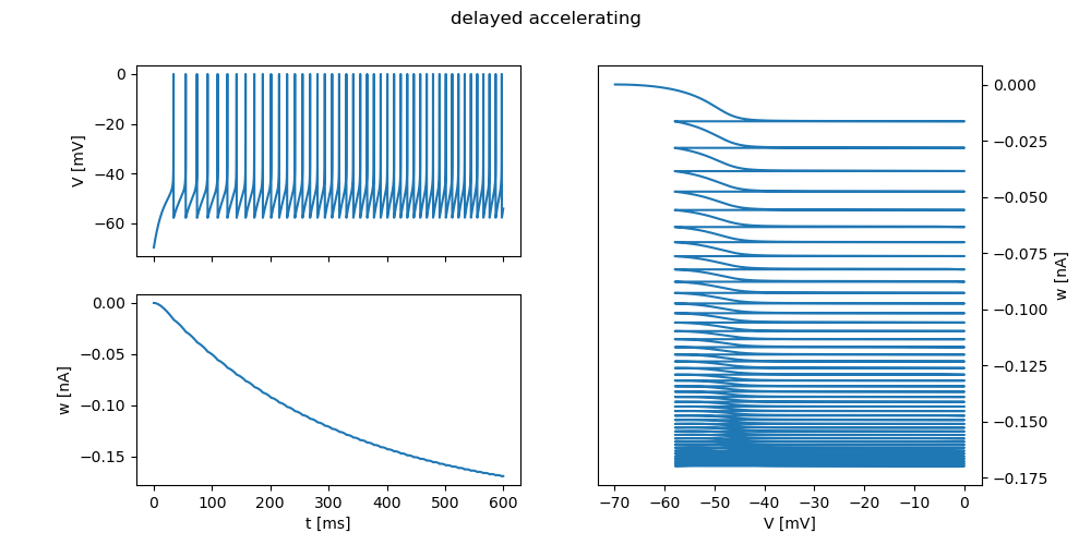
"delayed accelerating": {
"c_m": 200 * pF,
"g_l": 12 * nS,
"e_l": -70.0 * mV,
"v_t": -50.0 * mV,
"d_t": 2.0 * mV,
"a": -10.0 * nS,
"tau_w": 300.0 * ms,
"b": 0.0 * pA,
"v_r": -58.0 * mV,
"i_stim": 300 * pA,
},
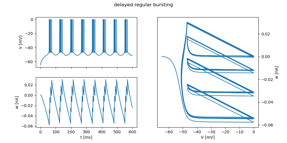
"delayed regular bursting": {
"c_m": 100 * pF,
"g_l": 10 * nS,
"e_l": -65.0 * mV,
"v_t": -50.0 * mV,
"d_t": 2.0 * mV,
"a": -10.0 * nS,
"tau_w": 90.0 * ms,
"b": 30.0 * pA,
"v_r": -47.0 * mV,
"i_stim": 110 * pA,
},
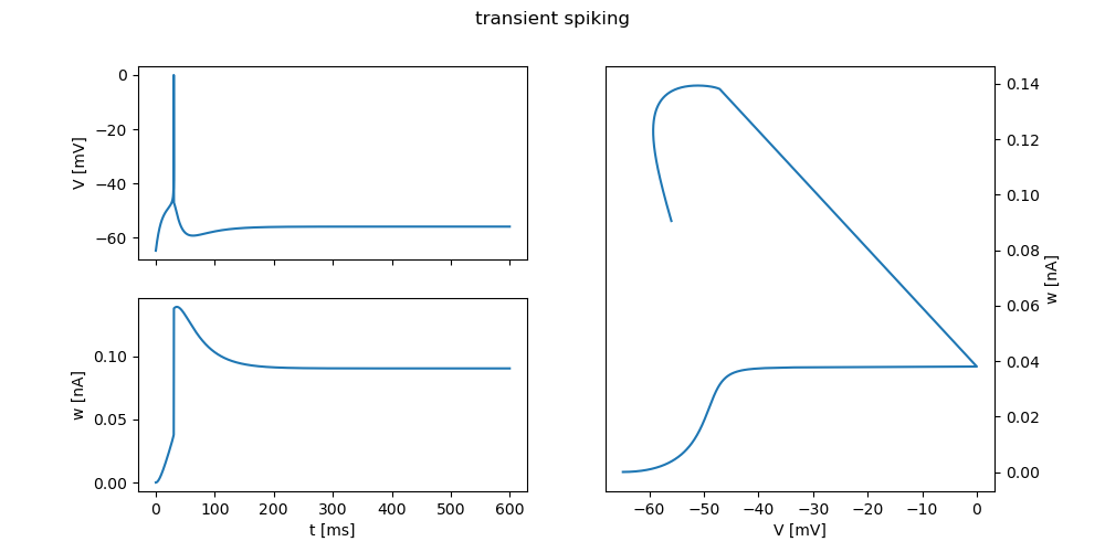
"transient spiking": {
"c_m": 100 * pF,
"g_l": 10 * nS,
"e_l": -65.0 * mV,
"v_t": -50.0 * mV,
"d_t": 2.0 * mV,
"a": 10.0 * nS,
"tau_w": 90.0 * ms,
"b": 100.0 * pA,
"v_r": -47.0 * mV,
"i_stim": 180 * pA,
},
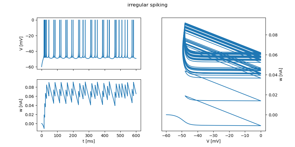
"irregular spiking": {
"c_m": 100 * pF,
"g_l": 12 * nS,
"e_l": -60.0 * mV,
"v_t": -50.0 * mV,
"d_t": 2.0 * mV,
"a": -11.0 * nS,
"tau_w": 130.0 * ms,
"b": 30.0 * pA,
"v_r": -48.0 * mV,
"i_stim": 160 * pA,
},
}
# loop over all patterns and plot
for pattern, parameters in patterns.items():
fig = plt.figure(figsize=(10, 5))
fig.suptitle(pattern)
gs = fig.add_gridspec(2, 2)
ax_vm = fig.add_subplot(gs[0, 0])
ax_w = fig.add_subplot(gs[1, 0])
ax_vm_w = fig.add_subplot(gs[:, 1])
sim(ax_vm, ax_w, ax_vm_w, parameters)
plt.show()