Example: Tetzlaff_2015

Note

You can launch an interactive, editable version of this example without installing any local files using the Binder service (although note that at some times this may be slow or fail to open):

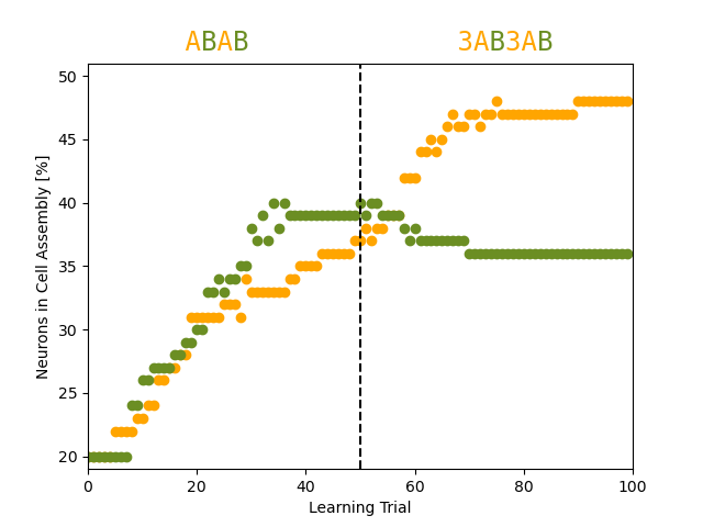
Reproduces Figure 2F of

The Use of Hebbian Cell Assemblies for Nonlinear Computation by Tetzlaff C., Dasgupta S., Kulvicius T. and Wörgötter F.

Sci Rep 5, 12866 (2015). https://doi.org/10.1038/srep12866

Sebastian Schmitt, 2022

import numpy as np
import matplotlib.pyplot as plt

from brian2 import NeuronGroup, Synapses, StateMonitor, run, defaultclock, ms, second, TimedArray, seed

# random seed that gives curves similar to the ones in the publication
seed(9873487)

# neuron parameters (sigmoidal activation)
beta = 0.03
epsilon = 120
F_max = 100
F_T = 1
tau_u = 1*ms
R = 0.012

# plasticity timescales
tau_ratio = 60
# hebbian
tau_H = 3e4*ms
# synaptic scaling
tau_SS = tau_ratio * tau_H

# synaptic weights
W_max = np.sqrt(tau_ratio*(F_max**2/(F_max - F_T)))
W_ext = W_max
W_input = W_max
W_I = 0.3*W_max

# stimulus
N_units = 100
N_stim_units = 20
stim_A_units_until = N_stim_units
stim_B_units_from = N_units-N_stim_units

# connection probabilities
p_E = 0.1
p_I = 0.2

# paper uses 0.3*ms
DT = 0.5*ms
defaultclock.dt = DT

# duration of a learning trial
lt = 5000*DT

duration = 100*lt
no_input_until = 5*lt
balanced_until = duration/2

# gate balanced presentation of stimulus 1 and 2
balanced = TimedArray([lt_counter*lt < balanced_until for lt_counter in range(int(duration/lt))], dt=lt)

# function used for stimulus (typo in paper, +1 is not part of the argument of sin)
stim_func = TimedArray([100*(np.sin(0.1*(i+1))+1) for i in range(int(duration/DT))], dt=DT)

# gate learning phase of either stimulus 1 or 2
learning_phase = TimedArray([i%10 > 3 for i in range(int(duration/(0.1*lt)))], dt=0.1*lt)

# if not balanced present stimulus A three times more often than stimulus B
stim_A_gate = TimedArray([lt_counter % 2 == 0 if balanced(lt_counter*lt) else lt_counter % 4 in [0,1,2]
                          for lt_counter in range(int(duration/lt))], dt=lt)

stim_B_gate = TimedArray([lt_counter % 2 == 1 if balanced(lt_counter*lt) else lt_counter % 4 == 3
                          for lt_counter in range(int(duration/lt))], dt=lt)

# noise is applied also during stimulation
neurons = NeuronGroup(N_units,
                      """
                      F = F_max/(1+exp(beta*(epsilon-u))) : 1
                      du/dt = (-u + R*(I_E - I_I + W_input*(I_stim_A + I_stim_B)))/tau_u + R*W_ext*20*sqrt((DT/ms)/ms)*xi: 1
                      I_E : 1
                      I_I : 1
                      index : 1 (constant)
                      stim_units_A = index < stim_A_units_until :  boolean
                      stim_units_B = index >= (stim_B_units_from) : boolean
                      I_stim_A = learning_phase(t)*int(stim_units_A)*stim_A_gate(t)*stim_func(t) : 1
                      I_stim_B = learning_phase(t)*int(stim_units_B)*stim_B_gate(t)*stim_func(t) : 1
                      """,
                      method = "euler")
neurons.index = range(len(neurons))

# excitatory connections with Hebbian plasticity and synaptic scaling
synapses_E = Synapses(neurons, neurons,
                      """
                      dw/dt = 1/tau_H*F_pre*F_post + 1/tau_SS*(F_T - F_post)*w**2 : 1 (clock-driven)
                      I_E_post = w*F_pre : 1 (summed)
                      """,
                      method="euler"
                      )
# do not connect between the two populations of stimulated neurons
synapses_E.connect(p=p_E, condition="((j > stim_A_units_until and i >= stim_B_units_from) or (j < stim_B_units_from and i < stim_A_units_until))"
                                    "or ((i > stim_A_units_until and i < stim_B_units_from) and (j > stim_A_units_until and j < stim_B_units_from))")

# fixed weight inhibitory connections
synapses_I = Synapses(neurons, neurons,
                      """
                      w : 1
                      I_I_post = w*F_pre : 1 (summed)
                      """
                      )
synapses_I.connect(p=p_I)
synapses_I.w = W_I

statemon_neurons = StateMonitor(neurons, ["F", "I_stim_A", "I_stim_B"], record=True, dt=100*defaultclock.dt)
statemon_synapses_E = StateMonitor(synapses_E, "w", record=True, dt=100*defaultclock.dt)
statemon_synapses_for_assembly_analysis = StateMonitor(synapses_E, "w", record=True, dt=lt)

run(duration, report="text")

# threshold saying that synaptic efficacies larger than theta are
# 'strong' and others are 'weak'
theta = 0.5*W_max

in_assembly_A = []
in_assembly_B = []

# traverse through the graph following 'strong' synapses
def go(W, source, units_in_assembly):
    units_in_assembly.add(source)
    # check all possible targets
    for target in range(N_units):
        w = W[source][target]
        if w > theta:
            W[source][target] = 0
            go(W, target, units_in_assembly)

# for each learning trial
for ws in statemon_synapses_for_assembly_analysis.w.T:

    # construct a full weight matrix
    W = np.full((N_units, N_units), np.nan)
    W[synapses_E.i[:], synapses_E.j[:]] = ws

    for in_assembly, stim_units in zip([in_assembly_A, in_assembly_B],
                                       [range(stim_A_units_until),
                                        range(stim_B_units_from, N_units)]):

        units_in_assembly = set()

        # start with units that are stimulated
        for stim_unit in stim_units:
            go(W, stim_unit, units_in_assembly)

        in_assembly.append(len(units_in_assembly))

# competitive development of the two competing cell assemblies A and B as a function of the input protocol
fig, ax = plt.subplots()

ax.plot(in_assembly_A, linestyle="None", marker='o', color='orange', label="A")
ax.plot(in_assembly_B, linestyle="None", marker='o', color='olivedrab', label="B")
ax.set_ylim(19, 51)
ax.set_xlim(0, 100)

ax.set_ylabel("Neurons in Cell Assembly [%]")
ax.set_xlabel("Learning Trial")

ax.axvline(balanced_until/lt, linestyle='dashed', color='k')

ax.text(15, 52, " A A", color='orange', fontfamily="monospace", fontsize="xx-large")
ax.text(15, 52, "  B B", color='olivedrab', fontfamily="monospace", fontsize="xx-large")

ax.text(65, 52, " 3A 3A", color='orange', fontfamily="monospace", fontsize="xx-large")
ax.text(65, 52, "   B  B", color='olivedrab', fontfamily="monospace", fontsize="xx-large")

plt.show()

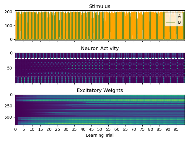
# stimulus, neuronal activity and excitatory weights as function of time
fig, axes = plt.subplots(3, sharex=True)

axes[0].plot(statemon_neurons.I_stim_A[0], label="A", color='orange')
axes[0].plot(statemon_neurons.I_stim_B[-1], label="B", color='olivedrab')
axes[0].legend(loc="upper right")
axes[0].set_title("Stimulus")

axes[1].imshow(statemon_neurons.F, aspect='auto')
axes[1].set_title("Neuron Activity")
axes[1].axhline(stim_A_units_until, linestyle='dashed', color='white')
axes[1].axhline(stim_B_units_from, linestyle='dashed', color='white')

axes[2].imshow(statemon_synapses_E.w, aspect='auto')
axes[2].set_title("Excitatory Weights")

axes[2].set_xticks(range(0, 5000, 250))
axes[2].set_xticklabels(f"{i}" for i in range(0, 100, 5))

axes[2].set_xlabel("Learning Trial")
axes[2].set_xlim(0, 5000)

fig.tight_layout()

plt.show()