Example: example_1_COBA
Note
You can launch an interactive, editable version of this example without installing any local files using the Binder service (although note that at some times this may be slow or fail to open):
Modeling neuron-glia interactions with the Brian 2 simulator Marcel Stimberg, Dan F. M. Goodman, Romain Brette, Maurizio De Pittà bioRxiv 198366; doi: https://doi.org/10.1101/198366
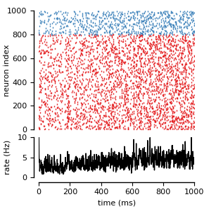
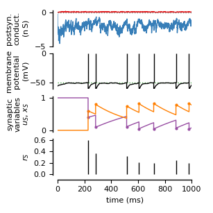
Figure 1: Modeling of neurons and synapses.
Randomly connected networks with conductance-based synapses (COBA; see Brunel, 2000). Synapses exhibit short-time plasticity (Tsodyks, 2005; Tsodyks et al., 1998).
from brian2 import *
import sympy

import plot_utils as pu

seed(11922)  # to get identical figures for repeated runs

################################################################################
# Model parameters
################################################################################
### General parameters
duration = 1.0*second  # Total simulation time
sim_dt = 0.1*ms        # Integrator/sampling step
N_e = 3200             # Number of excitatory neurons
N_i = 800              # Number of inhibitory neurons

### Neuron parameters
E_l = -60*mV           # Leak reversal potential
g_l = 9.99*nS          # Leak conductance
E_e = 0*mV             # Excitatory synaptic reversal potential
E_i = -80*mV           # Inhibitory synaptic reversal potential
C_m = 198*pF           # Membrane capacitance
tau_e = 5*ms           # Excitatory synaptic time constant
tau_i = 10*ms          # Inhibitory synaptic time constant
tau_r = 5*ms           # Refractory period
I_ex = 150*pA          # External current
V_th = -50*mV          # Firing threshold
V_r = E_l              # Reset potential

### Synapse parameters
w_e = 0.05*nS          # Excitatory synaptic conductance
w_i = 1.0*nS           # Inhibitory synaptic conductance
U_0 = 0.6              # Synaptic release probability at rest
Omega_d = 2.0/second   # Synaptic depression rate
Omega_f = 3.33/second  # Synaptic facilitation rate

################################################################################
# Model definition
################################################################################
# Set the integration time (in this case not strictly necessary, since we are
# using the default value)
defaultclock.dt = sim_dt

### Neurons
neuron_eqs = '''
dv/dt = (g_l*(E_l-v) + g_e*(E_e-v) + g_i*(E_i-v) +
         I_ex)/C_m    : volt (unless refractory)
dg_e/dt = -g_e/tau_e  : siemens  # post-synaptic exc. conductance
dg_i/dt = -g_i/tau_i  : siemens  # post-synaptic inh. conductance
'''
neurons = NeuronGroup(N_e + N_i, model=neuron_eqs,
                      threshold='v>V_th', reset='v=V_r',
                      refractory='tau_r', method='euler')
# Random initial membrane potential values and conductances
neurons.v = 'E_l + rand()*(V_th-E_l)'
neurons.g_e = 'rand()*w_e'
neurons.g_i = 'rand()*w_i'
exc_neurons = neurons[:N_e]
inh_neurons = neurons[N_e:]

### Synapses
synapses_eqs = '''
# Usage of releasable neurotransmitter per single action potential:
du_S/dt = -Omega_f * u_S     : 1 (event-driven)
# Fraction of synaptic neurotransmitter resources available:
dx_S/dt = Omega_d *(1 - x_S) : 1 (event-driven)
'''
synapses_action = '''
u_S += U_0 * (1 - u_S)
r_S = u_S * x_S
x_S -= r_S
'''
exc_syn = Synapses(exc_neurons, neurons, model=synapses_eqs,
                   on_pre=synapses_action+'g_e_post += w_e*r_S')
inh_syn = Synapses(inh_neurons, neurons, model=synapses_eqs,
                   on_pre=synapses_action+'g_i_post += w_i*r_S')

exc_syn.connect(p=0.05)
inh_syn.connect(p=0.2)
# Start from "resting" condition: all synapses have fully-replenished
# neurotransmitter resources
exc_syn.x_S = 1
inh_syn.x_S = 1

# ##############################################################################
# # Monitors
# ##############################################################################
# Note that we could use a single monitor for all neurons instead, but in this
# way plotting is a bit easier in the end
exc_mon = SpikeMonitor(exc_neurons)
inh_mon = SpikeMonitor(inh_neurons)

### We record some additional data from a single excitatory neuron
ni = 50
# Record conductances and membrane potential of neuron ni
state_mon = StateMonitor(exc_neurons, ['v', 'g_e', 'g_i'], record=ni)
# We make sure to monitor synaptic variables after synapse are updated in order
# to use simple recurrence relations to reconstruct them. Record all synapses
# originating from neuron ni
synapse_mon = StateMonitor(exc_syn, ['u_S', 'x_S'],
                           record=exc_syn[ni, :], when='after_synapses')

# ##############################################################################
# # Simulation run
# ##############################################################################
run(duration, report='text')

################################################################################
# Analysis and plotting
################################################################################
plt.style.use('figures.mplstyle')

### Spiking activity (w/ rate)
fig1, ax = plt.subplots(nrows=2, ncols=1, sharex=False,
                        gridspec_kw={'height_ratios': [3, 1],
                                     'left': 0.18, 'bottom': 0.18, 'top': 0.95,
                                     'hspace': 0.1},
                        figsize=(3.07, 3.07))
ax[0].plot(exc_mon.t[exc_mon.i <= N_e//4]/ms,
           exc_mon.i[exc_mon.i <= N_e//4], '|', color='C0')
ax[0].plot(inh_mon.t[inh_mon.i <= N_i//4]/ms,
           inh_mon.i[inh_mon.i <= N_i//4]+N_e//4, '|', color='C1')
pu.adjust_spines(ax[0], ['left'])
ax[0].set(xlim=(0., duration/ms), ylim=(0, (N_e+N_i)//4), ylabel='neuron index')

# Generate frequencies
bin_size = 1*ms
spk_count, bin_edges = np.histogram(np.r_[exc_mon.t/ms, inh_mon.t/ms],
                                    int(duration/ms))
rate = double(spk_count)/(N_e + N_i)/bin_size/Hz
ax[1].plot(bin_edges[:-1], rate, '-', color='k')
pu.adjust_spines(ax[1], ['left', 'bottom'])
ax[1].set(xlim=(0., duration/ms), ylim=(0, 10.),
          xlabel='time (ms)', ylabel='rate (Hz)')
pu.adjust_ylabels(ax, x_offset=-0.18)

### Dynamics of a single neuron
fig2, ax = plt.subplots(4, sharex=False,
                       gridspec_kw={'left': 0.27, 'bottom': 0.18, 'top': 0.95,
                                    'hspace': 0.2},
                       figsize=(3.07, 3.07))
### Postsynaptic conductances
ax[0].plot(state_mon.t/ms, state_mon.g_e[0]/nS, color='C0')
ax[0].plot(state_mon.t/ms, -state_mon.g_i[0]/nS, color='C1')
ax[0].plot([state_mon.t[0]/ms, state_mon.t[-1]/ms], [0, 0], color='grey',
           linestyle=':')
# Adjust axis
pu.adjust_spines(ax[0], ['left'])
ax[0].set(xlim=(0., duration/ms), ylim=(-5.0, 0.25),
          ylabel=f"postsyn.\nconduct.\n(${sympy.latex(nS)}$)")

### Membrane potential
ax[1].axhline(V_th/mV, color='C2', linestyle=':')  # Threshold
# Artificially insert spikes
ax[1].plot(state_mon.t/ms, state_mon.v[0]/mV, color='black')
ax[1].vlines(exc_mon.t[exc_mon.i == ni]/ms, V_th/mV, 0, color='black')
pu.adjust_spines(ax[1], ['left'])
ax[1].set(xlim=(0., duration/ms), ylim=(-1+V_r/mV, 0.),
          ylabel=f"membrane\npotential\n(${sympy.latex(mV)}$)")

### Synaptic variables
# Retrieves indexes of spikes in the synaptic monitor using the fact that we
# are sampling spikes and synaptic variables by the same dt
spk_index = np.in1d(synapse_mon.t, exc_mon.t[exc_mon.i == ni])
ax[2].plot(synapse_mon.t[spk_index]/ms, synapse_mon.x_S[0][spk_index], '.',
           ms=4, color='C3')
ax[2].plot(synapse_mon.t[spk_index]/ms, synapse_mon.u_S[0][spk_index], '.',
           ms=4, color='C4')
# Super-impose reconstructed solutions
time = synapse_mon.t  # time vector
tspk = Quantity(synapse_mon.t, copy=True)  # Spike times
for ts in exc_mon.t[exc_mon.i == ni]:
    tspk[time >= ts] = ts
ax[2].plot(synapse_mon.t/ms, 1 + (synapse_mon.x_S[0]-1)*exp(-(time-tspk)*Omega_d),
           '-', color='C3')
ax[2].plot(synapse_mon.t/ms, synapse_mon.u_S[0]*exp(-(time-tspk)*Omega_f),
           '-', color='C4')
# Adjust axis
pu.adjust_spines(ax[2], ['left'])
ax[2].set(xlim=(0., duration/ms), ylim=(-0.05, 1.05),
          ylabel='synaptic\nvariables\n$u_S,\,x_S$')

nspikes = np.sum(spk_index)
x_S_spike = synapse_mon.x_S[0][spk_index]
u_S_spike = synapse_mon.u_S[0][spk_index]
ax[3].vlines(synapse_mon.t[spk_index]/ms, np.zeros(nspikes),
             x_S_spike*u_S_spike/(1-u_S_spike))
pu.adjust_spines(ax[3], ['left', 'bottom'])
ax[3].set(xlim=(0., duration/ms), ylim=(-0.01, 0.62),
          yticks=np.arange(0, 0.62, 0.2), xlabel='time (ms)', ylabel='$r_S$')

pu.adjust_ylabels(ax, x_offset=-0.20)


plt.show()