Example: example_6_COBA_with_astro
Note
You can launch an interactive, editable version of this example without installing any local files using the Binder service (although note that at some times this may be slow or fail to open):
Modeling neuron-glia interactions with the Brian 2 simulator Marcel Stimberg, Dan F. M. Goodman, Romain Brette, Maurizio De Pittà bioRxiv 198366; doi: https://doi.org/10.1101/198366
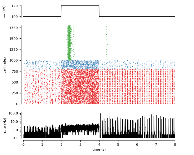
Figure 6: Recurrent neuron-glial network.
Randomly connected COBA network (see Brunel, 2000) with excitatory synapses modulated by release-increasing gliotransmission from a randomly connected network of astrocytes.
from brian2 import *

import plot_utils as pu

set_device('cpp_standalone', directory=None)  # Use fast "C++ standalone mode"
seed(28371)  # to get identical figures for repeated runs

################################################################################
# Model parameters
################################################################################
### General parameters
N_e = 3200                   # Number of excitatory neurons
N_i = 800                    # Number of inhibitory neurons
N_a = 3200                   # Number of astrocytes

## Some metrics parameters needed to establish proper connections
size = 3.75*mmeter           # Length and width of the square lattice
distance = 50*umeter         # Distance between neurons

### Neuron parameters
E_l = -60*mV                 # Leak reversal potential
g_l = 9.99*nS                # Leak conductance
E_e = 0*mV                   # Excitatory synaptic reversal potential
E_i = -80*mV                 # Inhibitory synaptic reversal potential
C_m = 198*pF                 # Membrane capacitance
tau_e = 5*ms                 # Excitatory synaptic time constant
tau_i = 10*ms                # Inhibitory synaptic time constant
tau_r = 5*ms                 # Refractory period
I_ex = 100*pA                # External current
V_th = -50*mV                # Firing threshold
V_r = E_l                    # Reset potential

### Synapse parameters
rho_c = 0.005                # Synaptic vesicle-to-extracellular space volume ratio
Y_T = 500.*mmolar            # Total vesicular neurotransmitter concentration
Omega_c = 40/second          # Neurotransmitter clearance rate
U_0__star = 0.6              # Resting synaptic release probability
Omega_f = 3.33/second        # Synaptic facilitation rate
Omega_d = 2.0/second         # Synaptic depression rate
w_e = 0.05*nS                # Excitatory synaptic conductance
w_i = 1.0*nS                 # Inhibitory synaptic conductance
# --- Presynaptic receptors
O_G = 1.5/umolar/second      # Agonist binding (activating) rate
Omega_G = 0.5/(60*second)    # Agonist release (deactivating) rate

### Astrocyte parameters
# ---  Calcium fluxes
O_P = 0.9*umolar/second      # Maximal Ca^2+ uptake rate by SERCAs
K_P = 0.05*umolar            # Ca2+ affinity of SERCAs
C_T = 2*umolar               # Total cell free Ca^2+ content
rho_A = 0.18                 # ER-to-cytoplasm volume ratio
Omega_C = 6/second           # Maximal rate of Ca^2+ release by IP_3Rs
Omega_L = 0.1/second         # Maximal rate of Ca^2+ leak from the ER
# --- IP_3R kinectics
d_1 = 0.13*umolar            # IP_3 binding affinity
d_2 = 1.05*umolar            # Ca^2+ inactivation dissociation constant
O_2 = 0.2/umolar/second      # IP_3R binding rate for Ca^2+ inhibition
d_3 = 0.9434*umolar          # IP_3 dissociation constant
d_5 = 0.08*umolar            # Ca^2+ activation dissociation constant
# --- IP_3 production
# --- Agonist-dependent IP_3 production
O_beta = 0.5*umolar/second   # Maximal rate of IP_3 production by PLCbeta
O_N = 0.3/umolar/second      # Agonist binding rate
Omega_N = 0.5/second         # Maximal inactivation rate
K_KC = 0.5*umolar            # Ca^2+ affinity of PKC
zeta = 10                    # Maximal reduction of receptor affinity by PKC
# --- Endogenous IP3 production
O_delta = 1.2*umolar/second  # Maximal rate of IP_3 production by PLCdelta
kappa_delta = 1.5*umolar     # Inhibition constant of PLC_delta by IP_3
K_delta = 0.1*umolar         # Ca^2+ affinity of PLCdelta
# --- IP_3 degradation
Omega_5P = 0.05/second       # Maximal rate of IP_3 degradation by IP-5P
K_D = 0.7*umolar             # Ca^2+ affinity of IP3-3K
K_3K = 1.0*umolar            # IP_3 affinity of IP_3-3K
O_3K = 4.5*umolar/second     # Maximal rate of IP_3 degradation by IP_3-3K
# --- IP_3 diffusion
F = 0.09*umolar/second       # GJC IP_3 permeability
I_Theta = 0.3*umolar         # Threshold gradient for IP_3 diffusion
omega_I = 0.05*umolar        # Scaling factor of diffusion
# --- Gliotransmitter release and time course
C_Theta = 0.5*umolar         # Ca^2+ threshold for exocytosis
Omega_A = 0.6/second         # Gliotransmitter recycling rate
U_A = 0.6                    # Gliotransmitter release probability
G_T = 200*mmolar             # Total vesicular gliotransmitter concentration
rho_e = 6.5e-4               # Astrocytic vesicle-to-extracellular volume ratio
Omega_e = 60/second          # Gliotransmitter clearance rate
alpha = 0.0                  # Gliotransmission nature

################################################################################
# Define HF stimulus
################################################################################
stimulus = TimedArray([1.0, 1.2, 1.0, 1.0], dt=2*second)

################################################################################
# Simulation time (based on the stimulus)
################################################################################
duration = 8*second          # Total simulation time

################################################################################
# Model definition
################################################################################
### Neurons
neuron_eqs = '''
dv/dt = (g_l*(E_l-v) + g_e*(E_e-v) + g_i*(E_i-v) + I_ex*stimulus(t))/C_m : volt (unless refractory)
dg_e/dt = -g_e/tau_e : siemens  # post-synaptic excitatory conductance
dg_i/dt = -g_i/tau_i : siemens  # post-synaptic inhibitory conductance
# Neuron position in space
x : meter (constant)
y : meter (constant)
'''
neurons = NeuronGroup(N_e + N_i, model=neuron_eqs,
                      threshold='v>V_th', reset='v=V_r',
                      refractory='tau_r', method='euler')
exc_neurons = neurons[:N_e]
inh_neurons = neurons[N_e:]
# Arrange excitatory neurons in a grid
N_rows = int(sqrt(N_e))
N_cols = N_e//N_rows
grid_dist = (size / N_cols)
exc_neurons.x = '(i // N_rows)*grid_dist - N_rows/2.0*grid_dist'
exc_neurons.y = '(i % N_rows)*grid_dist - N_cols/2.0*grid_dist'
# Random initial membrane potential values and conductances
neurons.v = 'E_l + rand()*(V_th-E_l)'
neurons.g_e = 'rand()*w_e'
neurons.g_i = 'rand()*w_i'

### Synapses
synapses_eqs = '''
# Neurotransmitter
dY_S/dt = -Omega_c * Y_S                                    : mmolar (clock-driven)
# Fraction of activated presynaptic receptors
dGamma_S/dt = O_G * G_A * (1 - Gamma_S) - Omega_G * Gamma_S : 1 (clock-driven)
# Usage of releasable neurotransmitter per single action potential:
du_S/dt = -Omega_f * u_S                                    : 1 (event-driven)
# Fraction of synaptic neurotransmitter resources available for release:
dx_S/dt = Omega_d *(1 - x_S)                                : 1 (event-driven)
U_0                                                         : 1
# released synaptic neurotransmitter resources:
r_S                                                         : 1
# gliotransmitter concentration in the extracellular space:
G_A                                                         : mmolar
# which astrocyte covers this synapse ?
astrocyte_index : integer (constant)
'''
synapses_action = '''
U_0 = (1 - Gamma_S) * U_0__star + alpha * Gamma_S
u_S += U_0 * (1 - u_S)
r_S = u_S * x_S
x_S -= r_S
Y_S += rho_c * Y_T * r_S
'''
exc_syn = Synapses(exc_neurons, neurons, model=synapses_eqs,
                   on_pre=synapses_action+'g_e_post += w_e*r_S',
                   method='exact')
exc_syn.connect(True, p=0.05)
exc_syn.x_S = 1.0
inh_syn = Synapses(inh_neurons, neurons, model=synapses_eqs,
                   on_pre=synapses_action+'g_i_post += w_i*r_S',
                   method='exact')
inh_syn.connect(True, p=0.2)
inh_syn.x_S = 1.0
# Connect excitatory synapses to an astrocyte depending on the position of the
# post-synaptic neuron
N_rows_a = int(sqrt(N_a))
N_cols_a = N_a/N_rows_a
grid_dist = size / N_rows_a
exc_syn.astrocyte_index = ('int(x_post/grid_dist) + '
                           'N_cols_a*int(y_post/grid_dist)')
### Astrocytes
# The astrocyte emits gliotransmitter when its Ca^2+ concentration crosses
# a threshold
astro_eqs = '''
# Fraction of activated astrocyte receptors:
dGamma_A/dt = O_N * Y_S * (1 - clip(Gamma_A,0,1)) -
              Omega_N*(1 + zeta * C/(C + K_KC)) * clip(Gamma_A,0,1) : 1
# Intracellular IP_3
dI/dt = J_beta + J_delta - J_3K - J_5P + J_coupling              : mmolar
J_beta = O_beta * Gamma_A                                        : mmolar/second
J_delta = O_delta/(1 + I/kappa_delta) * C**2/(C**2 + K_delta**2) : mmolar/second
J_3K = O_3K * C**4/(C**4 + K_D**4) * I/(I + K_3K)                : mmolar/second
J_5P = Omega_5P*I                                                : mmolar/second
# Diffusion between astrocytes:
J_coupling                                                       : mmolar/second

# Ca^2+-induced Ca^2+ release:
dC/dt = J_r + J_l - J_p                                   : mmolar
dh/dt = (h_inf - h)/tau_h                                 : 1
J_r = (Omega_C * m_inf**3 * h**3) * (C_T - (1 + rho_A)*C) : mmolar/second
J_l = Omega_L * (C_T - (1 + rho_A)*C)                     : mmolar/second
J_p = O_P * C**2/(C**2 + K_P**2)                          : mmolar/second
m_inf = I/(I + d_1) * C/(C + d_5)                         : 1
h_inf = Q_2/(Q_2 + C)                                     : 1
tau_h = 1/(O_2 * (Q_2 + C))                               : second
Q_2 = d_2 * (I + d_1)/(I + d_3)                           : mmolar

# Fraction of gliotransmitter resources available for release:
dx_A/dt = Omega_A * (1 - x_A) : 1
# gliotransmitter concentration in the extracellular space:
dG_A/dt = -Omega_e*G_A        : mmolar
# Neurotransmitter concentration in the extracellular space:
Y_S                           : mmolar
# The astrocyte position in space
x : meter (constant)
y : meter (constant)
'''
glio_release = '''
G_A += rho_e * G_T * U_A * x_A
x_A -= U_A *  x_A
'''
astrocytes = NeuronGroup(N_a, astro_eqs,
                         # The following formulation makes sure that a "spike" is
                         # only triggered at the first threshold crossing
                         threshold='C>C_Theta',
                         refractory='C>C_Theta',
                         # The gliotransmitter release happens when the threshold
                         # is crossed, in Brian terms it can therefore be
                         # considered a "reset"
                         reset=glio_release,
                         method='rk4',
                         dt=1e-2*second)
# Arrange astrocytes in a grid
astrocytes.x = '(i // N_rows_a)*grid_dist - N_rows_a/2.0*grid_dist'
astrocytes.y = '(i % N_rows_a)*grid_dist - N_cols_a/2.0*grid_dist'
# Add random initialization
astrocytes.C = 0.01*umolar
astrocytes.h = 0.9
astrocytes.I = 0.01*umolar
astrocytes.x_A = 1.0

ecs_astro_to_syn = Synapses(astrocytes, exc_syn,
                            'G_A_post = G_A_pre : mmolar (summed)')
ecs_astro_to_syn.connect('i == astrocyte_index_post')
ecs_syn_to_astro = Synapses(exc_syn, astrocytes,
                            'Y_S_post = Y_S_pre/N_incoming : mmolar (summed)')
ecs_syn_to_astro.connect('astrocyte_index_pre == j')
# Diffusion between astrocytes
astro_to_astro_eqs = '''
delta_I = I_post - I_pre            : mmolar
J_coupling_post = -(1 + tanh((abs(delta_I) - I_Theta)/omega_I))*
                  sign(delta_I)*F/2 : mmolar/second (summed)
'''
astro_to_astro = Synapses(astrocytes, astrocytes,
                          model=astro_to_astro_eqs)
# Connect to all astrocytes less than 75um away
# (about 4 connections per astrocyte)
astro_to_astro.connect('i != j and '
                       'sqrt((x_pre-x_post)**2 +'
                       '     (y_pre-y_post)**2) < 75*um')

################################################################################
# Monitors
################################################################################
# Note that we could use a single monitor for all neurons instead, but this
# way plotting is a bit easier in the end
exc_mon = SpikeMonitor(exc_neurons)
inh_mon = SpikeMonitor(inh_neurons)
ast_mon = SpikeMonitor(astrocytes)

################################################################################
# Simulation run
################################################################################
run(duration, report='text')

################################################################################
# Plot of Spiking activity
################################################################################
plt.style.use('figures.mplstyle')

fig, ax = plt.subplots(nrows=3, ncols=1, sharex=True, figsize=(6.26894, 6.26894*0.8),
                       gridspec_kw={'height_ratios': [1, 6, 2],
                                    'left': 0.12, 'top': 0.97})
time_range = np.linspace(0, duration/second, int(duration/second*100))*second
ax[0].plot(time_range, I_ex*stimulus(time_range)/pA, 'k')
ax[0].set(xlim=(0, duration/second), ylim=(98, 122),
          yticks=[100, 120], ylabel='$I_{ex}$ (pA)')
pu.adjust_spines(ax[0], ['left'])

## We only plot a fraction of the spikes
fraction = 4
ax[1].plot(exc_mon.t[exc_mon.i <= N_e//fraction]/second,
           exc_mon.i[exc_mon.i <= N_e//fraction], '|', color='C0')
ax[1].plot(inh_mon.t[inh_mon.i <= N_i//fraction]/second,
           inh_mon.i[inh_mon.i <= N_i//fraction]+N_e//fraction, '|', color='C1')
ax[1].plot(ast_mon.t[ast_mon.i <= N_a//fraction]/second,
           ast_mon.i[ast_mon.i <= N_a//fraction]+(N_e+N_i)//fraction,
           '|', color='C2')
ax[1].set(xlim=(0, duration/second), ylim=[0, (N_e+N_i+N_a)//fraction],
          yticks=np.arange(0, (N_e+N_i+N_a)//fraction+1, 250),
          ylabel='cell index')
pu.adjust_spines(ax[1], ['left'])

# Generate frequencies
bin_size = 1*ms
spk_count, bin_edges = np.histogram(np.r_[exc_mon.t/second, inh_mon.t/second],
                                    int(duration/bin_size))
rate = 1.0*spk_count/(N_e + N_i)/bin_size/Hz
rate[rate<0.001] = 0.001 # Fix 0 lower bound for log scale
ax[2].semilogy(bin_edges[:-1], rate, '-', color='k')
pu.adjust_spines(ax[2], ['left', 'bottom'])
ax[2].set(xlim=(0, duration/second), ylim=(0.1, 150),
          xticks=np.arange(0, 9), yticks=[0.1, 1, 10, 100],
          xlabel='time (s)', ylabel='rate (Hz)')
ax[2].get_yaxis().set_major_formatter(ScalarFormatter())

pu.adjust_ylabels(ax, x_offset=-0.11)

plt.show()