Example: Morris_Lecar_1981

Note

You can launch an interactive, editable version of this example without installing any local files using the Binder service (although note that at some times this may be slow or fail to open):

Morris-Lecar model

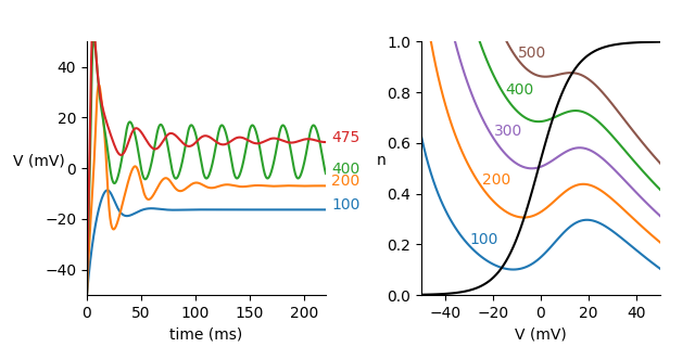
Reproduces Fig. 9 of:

Catherine Morris and Harold Lecar. “Voltage Oscillations in the Barnacle Giant Muscle Fiber.” Biophysical Journal 35, no. 1 (1981): 193–213.

from brian2 import *
set_device('cpp_standalone')
defaultclock.dt = 0.01*ms

g_L = 2*mS
g_Ca = 4*mS
g_K = 8*mS
V_L = -50*mV
V_Ca = 100*mV
V_K = -70*mV
lambda_n__max = 1.0/(15*ms)
V_1 = 10*mV
V_2 = 15*mV  # Note that Figure caption says -15 which seems to be a typo
V_3 = -1*mV
V_4 = 14.5*mV
C = 20*uF


# V,N-reduced system (Eq. 9 in article), note that the variables M and N (and lambda_N, etc.)
# have been renamed to m and n to better match the Hodgkin-Huxley convention, and because N has
# a reserved meaning in Brian (number of neurons)
eqs = '''
dV/dt = (-g_L*(V - V_L) - g_Ca*m_inf*(V - V_Ca) - g_K*n*(V - V_K) + I)/C : volt
dn/dt = lambda_n*(n_inf - n) : 1
m_inf = 0.5*(1 + tanh((V - V_1)/V_2)) : 1
n_inf = 0.5*(1 + tanh((V - V_3)/V_4)) : 1
lambda_n = lambda_n__max*cosh((V - V_3)/(2*V_4)) : Hz
I : amp
'''

neuron = NeuronGroup(17, eqs, method='exponential_euler')
neuron.I = (np.arange(17)*25+100)*uA
neuron.V = V_L
neuron.n = 'n_inf'
mon = StateMonitor(neuron, ['V', 'n'], record=True)

run_time = 220*ms
run(run_time)
fig, (ax1, ax2) = plt.subplots(1, 2, gridspec_kw={'right': 0.95, 'bottom': 0.15},
                               figsize=(6.4, 3.2))
fig.subplots_adjust(wspace=0.4)
for line_no, idx in enumerate([0, 4, 12, 15]):
    color = 'C%d' % line_no
    ax1.plot(mon.t/ms, mon.V[idx]/mV, color=color)
    ax1.text(225, mon.V[idx][-1]/mV, '%.0f' % (neuron.I[idx]/uA), color=color)
ax1.set(xlim=(0, 220), ylim=(-50, 50), xlabel='time (ms)')
ax1.set_ylabel('V (mV)', rotation=0)
ax1.spines['right'].set_visible(False)
ax1.spines['top'].set_visible(False)

# dV/dt nullclines
V = linspace(-50, 50, 100)*mV
for line_no, (idx, color) in enumerate([(0, 'C0'), (4, 'C1'), (8, 'C4'), (12, 'C2'), (16, 'C5')]):
    n_null = (g_L*(V - V_L) + g_Ca*0.5*(1 + tanh((V - V_1)/V_2))*(V - V_Ca) - neuron.I[idx])/(-g_K*(V - V_K))
    ax2.plot(V/mV, n_null, color=color)
    ax2.text(V[20+5*line_no]/mV, n_null[20+5*line_no]+0.01, '%.0f' % (neuron.I[idx]/uA), color=color)
# dn/dt nullcline
n_null = 0.5*(1 + tanh((V - V_3)/V_4))
ax2.plot(V/mV, n_null, color='k')
ax2.set(xlim=(-50, 50), ylim=(0, 1), xlabel='V (mV)')
ax2.set_ylabel('n', rotation=0)
ax2.spines['right'].set_visible(False)
ax2.spines['top'].set_visible(False)
plt.show()