Example: Wang_2002
Note
You can launch an interactive, editable version of this example without installing any local files using the Binder service (although note that at some times this may be slow or fail to open):
Decision network as in:
Wang, X.-J. Probabilistic decision making by slow reverberation in cortical circuits. Neuron, 2002, 36, 955-968.
Authors: Klaus Wimmer (kwimmer@crm.cat) and Marcel Stimberg
from brian2 import *
# -----------------------------------------------------------------------------------------------
# Set up the simulation
# -----------------------------------------------------------------------------------------------
# Stimulus and simulation parameters
coh = 12.8 # coherence of random dots
sigma = 4.0 * Hz # standard deviation of stimulus input
mu0 = 40.0 * Hz # stimulus input at zero coherence
mu1 = 40.0 * Hz # selective stimulus input at highest coherence
stim_interval = 50.0 * ms # stimulus changes every 50 ms
stim_on = 1000 * ms # stimulus onset
stim_off = 3000 * ms # stimulus offset
runtime = 4000 * ms # total simulation time
# External noise inputs
N_ext = 1000 # number of external Poisson neurons
rate_ext_E = 2400 * Hz / N_ext # external Poisson rate for excitatory population
rate_ext_I = 2400 * Hz / N_ext # external Poisson rate for inhibitory population
# Network parameters
N = 2000 # number of neurons
f_inh = 0.2 # fraction of inhibitory neurons
NE = int(N * (1.0 - f_inh)) # number of excitatory neurons (1600)
NI = int(N * f_inh) # number of inhibitory neurons (400)
fE = 0.15 # coding fraction
subN = int(fE * NE) # number of neurons in decision pools (240)
# Neuron parameters
El = -70.0 * mV # resting potential
Vt = -50.0 * mV # firing threshold
Vr = -55.0 * mV # reset potential
CmE = 0.5 * nF # membrane capacitance for pyramidal cells (excitatory neurons)
CmI = 0.2 * nF # membrane capacitance for interneurons (inhibitory neurons)
gLeakE = 25.0 * nS # membrane leak conductance of excitatory neurons
gLeakI = 20.0 * nS # membrane leak conductance of inhibitory neurons
refE = 2.0 * ms # refractory periodof excitatory neurons
refI = 1.0 * ms # refractory period of inhibitory neurons
# Synapse parameters
V_E = 0. * mV # reversal potential for excitatory synapses
V_I = -70. * mV # reversal potential for inhibitory synapses
tau_AMPA = 2.0 * ms # AMPA synapse decay
tau_NMDA_rise = 2.0 * ms # NMDA synapse rise
tau_NMDA_decay = 100.0 * ms # NMDA synapse decay
tau_GABA = 5.0 * ms # GABA synapse decay
alpha = 0.5 * kHz # saturation of NMDA channels at high presynaptic firing rates
C = 1 * mmole # extracellular magnesium concentration
# Synaptic conductances
gextE = 2.1 * nS # external -> excitatory neurons (AMPA)
gextI = 1.62 * nS # external -> inhibitory neurons (AMPA)
gEEA = 0.05 * nS / NE * 1600 # excitatory -> excitatory neurons (AMPA)
gEIA = 0.04 * nS / NE * 1600 # excitatory -> inhibitory neurons (AMPA)
gEEN = 0.165 * nS / NE * 1600 # excitatory -> excitatory neurons (NMDA)
gEIN = 0.13 * nS / NE * 1600 # excitatory -> inhibitory neurons (NMDA)
gIE = 1.3 * nS / NI * 400 # inhibitory -> excitatory neurons (GABA)
gII = 1.0 * nS / NI * 400 # inhibitory -> inhibitory neurons (GABA)
# Synaptic footprints
Jp = 1.7 # relative synaptic strength inside a selective population (1.0: no potentiation))
Jm = 1.0 - fE * (Jp - 1.0) / (1.0 - fE)
# Neuron equations
# Note the "(unless refractory)" statement serves to clamp the membrane voltage during the refractory period;
# otherwise the membrane potential continues to be integrated but no spikes are emitted.
eqsE = """
label : integer (constant) # label for decision encoding populations
dV/dt = (- gLeakE * (V - El) - I_AMPA - I_NMDA - I_GABA - I_AMPA_ext + I_input) / CmE : volt (unless refractory)
I_AMPA = s_AMPA * (V - V_E) : amp
ds_AMPA / dt = - s_AMPA / tau_AMPA : siemens
I_NMDA = gEEN * s_NMDA_tot * (V - V_E) / ( 1 + exp(-0.062 * V/mvolt) * (C/mmole / 3.57) ) : amp
s_NMDA_tot : 1
I_GABA = s_GABA * (V - V_I) : amp
ds_GABA / dt = - s_GABA / tau_GABA : siemens
I_AMPA_ext = s_AMPA_ext * (V - V_E) : amp
ds_AMPA_ext / dt = - s_AMPA_ext / tau_AMPA : siemens
I_input : amp
ds_NMDA / dt = - s_NMDA / tau_NMDA_decay + alpha * x * (1 - s_NMDA) : 1
dx / dt = - x / tau_NMDA_rise : 1
"""
eqsI = """
dV/dt = (- gLeakI * (V - El) - I_AMPA - I_NMDA - I_GABA - I_AMPA_ext) / CmI : volt (unless refractory)
I_AMPA = s_AMPA * (V - V_E) : amp
ds_AMPA / dt = - s_AMPA / tau_AMPA : siemens
I_NMDA = gEIN * s_NMDA_tot * (V - V_E) / ( 1 + exp(-0.062 * V/mvolt) * (C/mmole / 3.57) ): amp
s_NMDA_tot : 1
I_GABA = s_GABA * (V - V_I) : amp
ds_GABA / dt = - s_GABA / tau_GABA : siemens
I_AMPA_ext = s_AMPA_ext * (V - V_E) : amp
ds_AMPA_ext / dt = - s_AMPA_ext / tau_AMPA : siemens
"""
# Neuron populations
popE = NeuronGroup(NE, model=eqsE, threshold='V > Vt', reset='V = Vr', refractory=refE, method='euler', name='popE')
popI = NeuronGroup(NI, model=eqsI, threshold='V > Vt', reset='V = Vr', refractory=refI, method='euler', name='popI')
popE1 = popE[:subN]
popE2 = popE[subN:2 * subN]
popE3 = popE[2 * subN:]
popE1.label = 0
popE2.label = 1
popE3.label = 2
# Recurrent excitatory -> excitatory connections mediated by AMPA receptors
C_EE_AMPA = Synapses(popE, popE, 'w : siemens', on_pre='s_AMPA += w', delay=0.5 * ms, method='euler', name='C_EE_AMPA')
C_EE_AMPA.connect()
C_EE_AMPA.w[:] = gEEA
C_EE_AMPA.w["label_pre == label_post and label_pre < 2"] = gEEA*Jp
C_EE_AMPA.w["label_pre != label_post and label_post < 2"] = gEEA*Jm
# Note that this produces the following structure of excitatory connections:
#
# | from E1 from E2 from E3
# ---------------------------------
# to E1 | Jp Jm Jm
# to E2 | Jm Jp Jm
# to E3 | 1 1 1
# Recurrent excitatory -> inhibitory connections mediated by AMPA receptors
C_EI_AMPA = Synapses(popE, popI, on_pre='s_AMPA += gEIA', delay=0.5 * ms, method='euler', name='C_EI_AMPA')
C_EI_AMPA.connect()
# Recurrent excitatory -> excitatory connections mediated by NMDA receptors
C_EE_NMDA = Synapses(popE, popE, on_pre='x_pre += 1', delay=0.5 * ms, method='euler', name='C_EE_NMDA')
C_EE_NMDA.connect(j='i')
# Dummy population to store the summed activity of the three populations
NMDA_sum_group = NeuronGroup(3, 's : 1', name='NMDA_sum_group')
# Sum the activity according to the subpopulation labels
NMDA_sum = Synapses(popE, NMDA_sum_group, 's_post = s_NMDA_pre : 1 (summed)', name='NMDA_sum')
NMDA_sum.connect(j='label_pre')
# Propagate the summed activity to the NMDA synapses
NMDA_set_total_E = Synapses(NMDA_sum_group, popE,
'''w : 1 (constant)
s_NMDA_tot_post = w*s_pre : 1 (summed)''', name='NMDA_set_total_E')
NMDA_set_total_E.connect()
NMDA_set_total_E.w = 1
NMDA_set_total_E.w["i == label_post and label_post < 2"] = Jp
NMDA_set_total_E.w["i != label_post and label_post < 2"] = Jm
# Recurrent excitatory -> inhibitory connections mediated by NMDA receptors
NMDA_set_total_I = Synapses(NMDA_sum_group, popI,
'''s_NMDA_tot_post = s_pre : 1 (summed)''', name='NMDA_set_total_I')
NMDA_set_total_I.connect()
# Recurrent inhibitory -> excitatory connections mediated by GABA receptors
C_IE = Synapses(popI, popE, on_pre='s_GABA += gIE', delay=0.5 * ms, method='euler', name='C_IE')
C_IE.connect()
# Recurrent inhibitory -> inhibitory connections mediated by GABA receptors
C_II = Synapses(popI, popI, on_pre='s_GABA += gII', delay=0.5 * ms, method='euler', name='C_II')
C_II.connect()
# External inputs (fixed background firing rates)
extinputE = PoissonInput(popE, 's_AMPA_ext', N_ext, rate_ext_E, gextE)
extinputI = PoissonInput(popI, 's_AMPA_ext', N_ext, rate_ext_I, gextI)
# Stimulus input (updated every 50ms)
stiminputE1 = PoissonGroup(subN, rates=0*Hz, name='stiminputE1')
stiminputE2 = PoissonGroup(subN, rates=0*Hz, name='stiminputE2')
stiminputE1.run_regularly("rates = int(t > stim_on and t < stim_off) * (mu0 + coh / 100.0 * mu1 + sigma*randn())", dt=stim_interval)
stiminputE2.run_regularly("rates = int(t > stim_on and t < stim_off) * (mu0 - coh / 100.0 * mu1 + sigma*randn())", dt=stim_interval)
C_stimE1 = Synapses(stiminputE1, popE1, on_pre='s_AMPA_ext += gextE', name='C_stimE1')
C_stimE1.connect(j='i')
C_stimE2 = Synapses(stiminputE2, popE2, on_pre='s_AMPA_ext += gextE', name='C_stimE2')
C_stimE2.connect(j='i')
# -----------------------------------------------------------------------------------------------
# Run the simulation
# -----------------------------------------------------------------------------------------------
# Set initial conditions
popE.s_NMDA_tot = tau_NMDA_decay * 10 * Hz * 0.2
popI.s_NMDA_tot = tau_NMDA_decay * 10 * Hz * 0.2
popE.V = Vt - 2 * mV
popI.V = Vt - 2 * mV
# Record spikes of excitatory neurons in the decision encoding populations
SME1 = SpikeMonitor(popE1, record=True)
SME2 = SpikeMonitor(popE2, record=True)
# Record population activity
R1 = PopulationRateMonitor(popE1)
R2 = PopulationRateMonitor(popE2)
# Record input
E1 = StateMonitor(stiminputE1, 'rates', record=0, dt=1*ms)
E2 = StateMonitor(stiminputE2, 'rates', record=0, dt=1*ms)
# Run the simulation
run(runtime, report='stdout', profile=True)
print(profiling_summary())
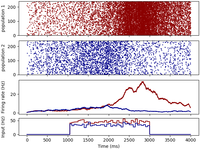
# Show results
fig, axs = plt.subplots(4, 1, sharex=True, layout='constrained', gridspec_kw={'height_ratios': [2, 2, 2, 1]})
axs[0].plot(SME1.t / ms, SME1.i, '.', markersize=2, color='darkred')
axs[0].set(ylabel='population 1', ylim=(0, subN))
axs[1].plot(SME2.t / ms, SME2.i, '.', markersize=2, color='darkblue')
axs[1].set(ylabel='population 2', ylim=(0, subN))
axs[2].plot(R1.t / ms, R1.smooth_rate(window='flat', width=100 * ms) / Hz, color='darkred')
axs[2].plot(R2.t / ms, R2.smooth_rate(window='flat', width=100 * ms) / Hz, color='darkblue')
axs[2].set(ylabel='Firing rate (Hz)')
axs[3].plot(E1.t / ms, E1.rates[0] / Hz, color='darkred')
axs[3].plot(E2.t / ms, E2.rates[0] / Hz, color='darkblue')
axs[3].set(ylabel='Input (Hz)', xlabel='Time (ms)')
fig.align_ylabels(axs)
plt.show()