Example: example_3_bisection
Note
You can launch an interactive, editable version of this example without installing any local files using the Binder service (although note that at some times this may be slow or fail to open):
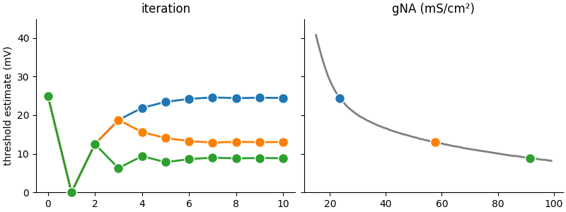
Reproduces Figure 4B from Stimberg et al. (2019).
Same code as in the https://github.com/brian-team/brian2_paper_examples repository, but using matplotlib instead of Plotly for plotting.
Marcel Stimberg, Romain Brette, Dan FM Goodman (2019) Brian 2, an intuitive and efficient neural simulator eLife 8:e47314
https://doi.org/10.7554/eLife.47314
from brian2 import *

defaultclock.dt = 0.01*ms  # small time step for stiff equations

# Our model of the neuron is based on the classical model of from Hodgkin and Huxley (1952). Note that this is not
# actually a model of a neuron, but rather of a (space-clamped) axon. However, to avoid confusion with spatially
# extended models, we simply use the term "neuron" here. In this model, the membrane potential is shifted, i.e. the
# resting potential is at 0mV:
El = 10.613*mV
ENa = 115*mV
EK = -12*mV
gl = 0.3*msiemens/cm**2
gK = 36*msiemens/cm**2
gNa_max = 100*msiemens/cm**2
gNa_min = 15*msiemens/cm**2
C = 1*uF/cm**2

eqs = """
dv/dt = (gl * (El-v) + gNa * m**3 * h * (ENa-v) + gK * n**4 * (EK-v)) / C : volt
gNa : siemens/meter**2 (constant)
dm/dt = alpham * (1-m) - betam * m : 1
dn/dt = alphan * (1-n) - betan * n : 1
dh/dt = alphah * (1-h) - betah * h : 1
alpham = (0.1/mV) * 10*mV / exprel((-v+25*mV) / (10*mV))/ms : Hz
betam = 4 * exp(-v/(18*mV))/ms : Hz
alphah = 0.07 * exp(-v/(20*mV))/ms : Hz
betah = 1/(exp((-v+30*mV) / (10*mV)) + 1)/ms : Hz
alphan = (0.01/mV) * 10*mV / exprel((-v+10*mV) / (10*mV))/ms : Hz
betan = 0.125*exp(-v/(80*mV))/ms : Hz
"""

# We simulate 100 neurons at the same time, each of them having a density of sodium channels between 15 and 100 mS/cm²:
neurons = NeuronGroup(100, eqs, method="rk4", threshold="v>50*mV", reset="")
neurons.gNa = "gNa_min + (gNa_max - gNa_min)*1.0*i/N"

# We initialize the state variables to their resting state values, note that the values for $m$, $n$, $h$ depend on the
# values of $\alpha_m$, $\beta_m$, etc. which themselves depend on $v$. The order of the assignments ($v$ is
# initialized before $m$, $n$, and $h$) therefore matters, something that is naturally expressed by stating initial
# values as sequential assignments to the state variables. In a declarative approach, this would be potentially
# ambiguous.

neurons.v = 0*mV
neurons.m = "1/(1 + betam/alpham)"
neurons.n = "1/(1 + betan/alphan)"
neurons.h = "1/(1 + betah/alphah)"

# We record the spiking activity of the neurons and store the current network state so that we can later restore it and
# run another iteration of our experiment:

S = SpikeMonitor(neurons)
store()

# The algorithm we use here to find the voltage threshold is a simple bisection: we try to find the threshold voltage of
# a neuron by repeatedly testing values and increasing or decreasing these values depending on whether we observe a
# spike or not. By continously halving the size of the correction, we quickly converge to a precise estimate.
#
# We start with the same initial estimate for all segments, 25mV above the resting potential, and the same value for
# the size of the "correction step":

v0 = 25*mV*np.ones(len(neurons))
step = 25*mV

# For later visualization of how the estimates converged towards their final values, we also store the intermediate values of the estimates:
estimates = np.full((11, len(neurons)), np.nan)*mV
estimates[0, :] = v0

# We now run 10 iterations of our algorithm:

for i in range(10):
    print(".", end="")
    # Reset to the initial state
    restore()
    # Set the membrane potential to our threshold estimate and update the initial values of the gating variables
    neurons.v = v0
    # Note that we do not update the initial values of the gating variables to their steady state values with
    # respect to v, but rather to the resting potential.
    # Run the simulation for 20ms
    run(20*ms)
    print()
    # Decrease the estimates for neurons that spiked
    v0[S.count > 0] -= step
    # Increase the estimate for neurons that did not spike
    v0[S.count == 0] += step
    # Reduce step size and store current estimate
    step /= 2.0
    estimates[i + 1, :] = v0
print()

# After the 10 iteration steps, we plot the results:
plt.rcParams.update({'axes.spines.top': False,
                     'axes.spines.right': False})
fig, (ax1, ax2) = plt.subplots(1, 2, sharey=True, figsize=(8, 3), layout="constrained")

colors = ["#1f77b4", "#ff7f03", "#2ca02c"]
examples = [10, 50, 90]
for example, color in zip(examples, colors):
    ax1.plot(np.arange(11), estimates[:, example] / mV,
             "o-", mec='white', lw=2, color=color, clip_on=False, ms=10, zorder=100,
             label=f"gNA = {(neurons.gNa[example]/(mS/cm**2)):.1f}mS/cm$^2$")

ax2.plot(neurons.gNa/(mS/cm**2), v0/mV, color="gray", lw=2)

for idx, (example, color) in enumerate(zip(examples, colors)):
    ax2.plot([neurons.gNa[example]/(mS/cm**2)], [estimates[-1, example]/mV], "o", color=color, mec="white", ms=10,
             label=f"gNA = {(neurons.gNa[example]/(mS/cm**2)):.1f}mS/cm$^2$")

ax1.set(title="iteration", ylim=(0, 45), ylabel="threshold estimate (mV)")
ax2.set(title="gNA (mS/cm²)")

plt.show()