Example: Touboul_Brette_2008
Note
You can launch an interactive, editable version of this example without installing any local files using the Binder service (although note that at some times this may be slow or fail to open):
Chaos in the AdEx model
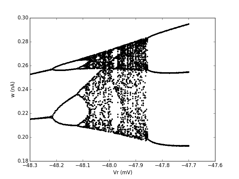
Fig. 8B from: Touboul, J. and Brette, R. (2008). Dynamics and bifurcations of the adaptive exponential integrate-and-fire model. Biological Cybernetics 99(4-5):319-34.
This shows the bifurcation structure when the reset value is varied (vertical axis shows the values of w at spike times for a given a reset value Vr).
from brian2 import *

defaultclock.dt = 0.01*ms

C = 281*pF
gL = 30*nS
EL = -70.6*mV
VT = -50.4*mV
DeltaT = 2*mV
tauw = 40*ms
a = 4*nS
b = 0.08*nA
I = .8*nA
Vcut = VT + 5 * DeltaT  # practical threshold condition
N = 200

eqs = """
dvm/dt=(gL*(EL-vm)+gL*DeltaT*exp((vm-VT)/DeltaT)+I-w)/C : volt
dw/dt=(a*(vm-EL)-w)/tauw : amp
Vr:volt
"""

neuron = NeuronGroup(N, model=eqs, threshold='vm > Vcut',
                     reset="vm = Vr; w += b", method='euler')
neuron.vm = EL
neuron.w = a * (neuron.vm - EL)
neuron.Vr = linspace(-48.3 * mV, -47.7 * mV, N)  # bifurcation parameter

init_time = 3*second
run(init_time, report='text')  # we discard the first spikes

states = StateMonitor(neuron, "w", record=True, when='start')
spikes = SpikeMonitor(neuron)
run(1 * second, report='text')

# Get the values of Vr and w for each spike
Vr = neuron.Vr[spikes.i]
w = states.w[spikes.i, int_((spikes.t-init_time)/defaultclock.dt)]

figure()
plot(Vr / mV, w / nA, '.k')
xlabel('Vr (mV)')
ylabel('w (nA)')
show()