Introduction to Brian part 1: Neurons
Note
This tutorial is a static non-editable version. You can launch an
interactive, editable version without installing any local files
using the Binder service (although note that at some times this
may be slow or fail to open): ![]()
Alternatively, you can download a copy of the notebook file
to use locally: 1-intro-to-brian-neurons.ipynb
See the tutorial overview page for more details.
All Brian scripts start with the following. If you’re trying this notebook out in the Jupyter notebook, you should start by running this cell.
from brian2 import *
Later we’ll do some plotting in the notebook, so we activate inline plotting in the notebook by doing this:
%matplotlib inline
If you are not using the Jupyter notebook to run this example (e.g. you
are using a standard Python terminal, or you copy&paste these example
into an editor and run them as a script), then plots will not
automatically be displayed. In this case, call the show() command
explicitly after the plotting commands.
Units system
Brian has a system for using quantities with physical dimensions:
20*volt
All of the basic SI units can be used (volt, amp, etc.) along with all
the standard prefixes (m=milli, p=pico, etc.), as well as a few special
abbreviations like mV for millivolt, pF for picofarad, etc.
1000*amp
1e6*volt
1000*namp
Also note that combinations of units with work as expected:
10*nA*5*Mohm
And if you try to do something wrong like adding amps and volts, what happens?
5*amp+10*volt
---------------------------------------------------------------------------

DimensionMismatchError                    Traceback (most recent call last)

<ipython-input-8-245c0c0332d1> in <module>
----> 1 5*amp+10*volt


~/programming/brian2/brian2/units/fundamentalunits.py in __add__(self, other)
   1429
   1430     def __add__(self, other):
-> 1431         return self._binary_operation(other, operator.add,
   1432                                       fail_for_mismatch=True,
   1433                                       operator_str='+')


~/programming/brian2/brian2/units/fundamentalunits.py in _binary_operation(self, other, operation, dim_operation, fail_for_mismatch, operator_str, inplace)
   1369                 message = ('Cannot calculate {value1} %s {value2}, units do not '
   1370                            'match') % operator_str
-> 1371                 _, other_dim = fail_for_dimension_mismatch(self, other, message,
   1372                                                            value1=self,
   1373                                                            value2=other)


~/programming/brian2/brian2/units/fundamentalunits.py in fail_for_dimension_mismatch(obj1, obj2, error_message, **error_quantities)
    184             raise DimensionMismatchError(error_message, dim1)
    185         else:
--> 186             raise DimensionMismatchError(error_message, dim1, dim2)
    187     else:
    188         return dim1, dim2


DimensionMismatchError: Cannot calculate 5. A + 10. V, units do not match (units are A and V).
If you haven’t see an error message in Python before that can look a bit overwhelming, but it’s actually quite simple and it’s important to know how to read these because you’ll probably see them quite often.
You should start at the bottom and work up. The last line gives the
error type DimensionMismatchError along with a more specific message
(in this case, you were trying to add together two quantities with
different SI units, which is impossible).
Working upwards, each of the sections starts with a filename
(e.g. C:\Users\Dan\...) with possibly the name of a function, and
then a few lines surrounding the line where the error occurred (which is
identified with an arrow).
The last of these sections shows the place in the function where the error actually happened. The section above it shows the function that called that function, and so on until the first section will be the script that you actually run. This sequence of sections is called a traceback, and is helpful in debugging.
If you see a traceback, what you want to do is start at the bottom and scan up the sections until you find your own file because that’s most likely where the problem is. (Of course, your code might be correct and Brian may have a bug in which case, please let us know on the email support list.)
A simple model
Let’s start by defining a simple neuron model. In Brian, all models are defined by systems of differential equations. Here’s a simple example of what that looks like:
tau = 10*ms
eqs = '''
dv/dt = (1-v)/tau : 1
'''
In Python, the notation ''' is used to begin and end a multi-line
string. So the equations are just a string with one line per equation.
The equations are formatted with standard mathematical notation, with
one addition. At the end of a line you write : unit where unit
is the SI unit of that variable. Note that this is not the unit of the
two sides of the equation (which would be 1/second), but the unit of
the variable defined by the equation, i.e. in this case \(v\).
Now let’s use this definition to create a neuron.
G = NeuronGroup(1, eqs)
In Brian, you only create groups of neurons, using the class
NeuronGroup. The first two arguments when you create one of these
objects are the number of neurons (in this case, 1) and the defining
differential equations.
Let’s see what happens if we didn’t put the variable tau in the
equation:
eqs = '''
dv/dt = 1-v : 1
'''
G = NeuronGroup(1, eqs)
run(100*ms)
---------------------------------------------------------------------------

DimensionMismatchError                    Traceback (most recent call last)

~/programming/brian2/brian2/equations/equations.py in check_units(self, group, run_namespace)
    955                 try:
--> 956                     check_dimensions(str(eq.expr), self.dimensions[var] / second.dim,
    957                                      all_variables)


~/programming/brian2/brian2/equations/unitcheck.py in check_dimensions(expression, dimensions, variables)
     44                                                   expected=repr(get_unit(dimensions)))
---> 45     fail_for_dimension_mismatch(expr_dims, dimensions, err_msg)
     46


~/programming/brian2/brian2/units/fundamentalunits.py in fail_for_dimension_mismatch(obj1, obj2, error_message, **error_quantities)
    183         if obj2 is None or isinstance(obj2, (Dimension, Unit)):
--> 184             raise DimensionMismatchError(error_message, dim1)
    185         else:


DimensionMismatchError: Expression 1-v does not have the expected unit hertz (unit is 1).


During handling of the above exception, another exception occurred:


DimensionMismatchError                    Traceback (most recent call last)

~/programming/brian2/brian2/core/network.py in before_run(self, run_namespace)
    897                 try:
--> 898                     obj.before_run(run_namespace)
    899                 except Exception as ex:


~/programming/brian2/brian2/groups/neurongroup.py in before_run(self, run_namespace)
    883         # Check units
--> 884         self.equations.check_units(self, run_namespace=run_namespace)
    885         # Check that subexpressions that refer to stateful functions are labeled


~/programming/brian2/brian2/equations/equations.py in check_units(self, group, run_namespace)
    958                 except DimensionMismatchError as ex:
--> 959                     raise DimensionMismatchError(('Inconsistent units in '
    960                                                   'differential equation '


DimensionMismatchError: Inconsistent units in differential equation defining variable v:
Expression 1-v does not have the expected unit hertz (unit is 1).


During handling of the above exception, another exception occurred:


BrianObjectException                      Traceback (most recent call last)

<ipython-input-11-97ed109f5888> in <module>
      3 '''
      4 G = NeuronGroup(1, eqs)
----> 5 run(100*ms)


~/programming/brian2/brian2/units/fundamentalunits.py in new_f(*args, **kwds)
   2383                                                      get_dimensions(newkeyset[k]))
   2384
-> 2385             result = f(*args, **kwds)
   2386             if 'result' in au:
   2387                 if au['result'] == bool:


~/programming/brian2/brian2/core/magic.py in run(duration, report, report_period, namespace, profile, level)
    371         intended use. See `MagicNetwork` for more details.
    372     '''
--> 373     return magic_network.run(duration, report=report, report_period=report_period,
    374                              namespace=namespace, profile=profile, level=2+level)
    375 run.__module__ = __name__


~/programming/brian2/brian2/core/magic.py in run(self, duration, report, report_period, namespace, profile, level)
    229             namespace=None, profile=False, level=0):
    230         self._update_magic_objects(level=level+1)
--> 231         Network.run(self, duration, report=report, report_period=report_period,
    232                     namespace=namespace, profile=profile, level=level+1)
    233


~/programming/brian2/brian2/core/base.py in device_override_decorated_function(*args, **kwds)
    274                 return getattr(curdev, name)(*args, **kwds)
    275             else:
--> 276                 return func(*args, **kwds)
    277
    278         device_override_decorated_function.__doc__ = func.__doc__


~/programming/brian2/brian2/units/fundamentalunits.py in new_f(*args, **kwds)
   2383                                                      get_dimensions(newkeyset[k]))
   2384
-> 2385             result = f(*args, **kwds)
   2386             if 'result' in au:
   2387                 if au['result'] == bool:


~/programming/brian2/brian2/core/network.py in run(self, duration, report, report_period, namespace, profile, level)
   1007             namespace = get_local_namespace(level=level+3)
   1008
-> 1009         self.before_run(namespace)
   1010
   1011         if len(all_objects) == 0:


~/programming/brian2/brian2/core/base.py in device_override_decorated_function(*args, **kwds)
    274                 return getattr(curdev, name)(*args, **kwds)
    275             else:
--> 276                 return func(*args, **kwds)
    277
    278         device_override_decorated_function.__doc__ = func.__doc__


~/programming/brian2/brian2/core/network.py in before_run(self, run_namespace)
    898                     obj.before_run(run_namespace)
    899                 except Exception as ex:
--> 900                     raise brian_object_exception("An error occurred when preparing an object.", obj, ex)
    901
    902         # Check that no object has been run as part of another network before


BrianObjectException: Original error and traceback:
Traceback (most recent call last):
  File "/home/marcel/programming/brian2/brian2/equations/equations.py", line 956, in check_units
    check_dimensions(str(eq.expr), self.dimensions[var] / second.dim,
  File "/home/marcel/programming/brian2/brian2/equations/unitcheck.py", line 45, in check_dimensions
    fail_for_dimension_mismatch(expr_dims, dimensions, err_msg)
  File "/home/marcel/programming/brian2/brian2/units/fundamentalunits.py", line 184, in fail_for_dimension_mismatch
    raise DimensionMismatchError(error_message, dim1)
brian2.units.fundamentalunits.DimensionMismatchError: Expression 1-v does not have the expected unit hertz (unit is 1).

During handling of the above exception, another exception occurred:

Traceback (most recent call last):
  File "/home/marcel/programming/brian2/brian2/core/network.py", line 898, in before_run
    obj.before_run(run_namespace)
  File "/home/marcel/programming/brian2/brian2/groups/neurongroup.py", line 884, in before_run
    self.equations.check_units(self, run_namespace=run_namespace)
  File "/home/marcel/programming/brian2/brian2/equations/equations.py", line 959, in check_units
    raise DimensionMismatchError(('Inconsistent units in '
brian2.units.fundamentalunits.DimensionMismatchError: Inconsistent units in differential equation defining variable v:
Expression 1-v does not have the expected unit hertz (unit is 1).

Error encountered with object named "neurongroup_1".
Object was created here (most recent call only, full details in debug log):
  File "<ipython-input-11-97ed109f5888>", line 4, in <module>
    G = NeuronGroup(1, eqs)

An error occurred when preparing an object. brian2.units.fundamentalunits.DimensionMismatchError: Inconsistent units in differential equation defining variable v:
Expression 1-v does not have the expected unit hertz (unit is 1).
(See above for original error message and traceback.)
An error is raised, but why? The reason is that the differential
equation is now dimensionally inconsistent. The left hand side dv/dt
has units of 1/second but the right hand side 1-v is
dimensionless. People often find this behaviour of Brian confusing
because this sort of equation is very common in mathematics. However,
for quantities with physical dimensions it is incorrect because the
results would change depending on the unit you measured it in. For time,
if you measured it in seconds the same equation would behave differently
to how it would if you measured time in milliseconds. To avoid this, we
insist that you always specify dimensionally consistent equations.
Now let’s go back to the good equations and actually run the simulation.
start_scope()

tau = 10*ms
eqs = '''
dv/dt = (1-v)/tau : 1
'''

G = NeuronGroup(1, eqs)
run(100*ms)
INFO No numerical integration method specified for group 'neurongroup', using method 'exact' (took 0.02s). [brian2.stateupdaters.base.method_choice]
First off, ignore that start_scope() at the top of the cell. You’ll
see that in each cell in this tutorial where we run a simulation. All it
does is make sure that any Brian objects created before the function is
called aren’t included in the next run of the simulation.
Secondly, you’ll see that there is an “INFO” message about not specifying the numerical integration method. This is harmless and just to let you know what method we chose, but we’ll fix it in the next cell by specifying the method explicitly.
So, what has happened here? Well, the command run(100*ms) runs the
simulation for 100 ms. We can see that this has worked by printing the
value of the variable v before and after the simulation.
start_scope()

G = NeuronGroup(1, eqs, method='exact')
print('Before v = %s' % G.v[0])
run(100*ms)
print('After v = %s' % G.v[0])
Before v = 0.0
After v = 0.9999546000702376
By default, all variables start with the value 0. Since the differential
equation is dv/dt=(1-v)/tau we would expect after a while that v
would tend towards the value 1, which is just what we see. Specifically,
we’d expect v to have the value 1-exp(-t/tau). Let’s see if
that’s right.
print('Expected value of v = %s' % (1-exp(-100*ms/tau)))
Expected value of v = 0.9999546000702375
Good news, the simulation gives the value we’d expect!
Now let’s take a look at a graph of how the variable v evolves over
time.
start_scope()

G = NeuronGroup(1, eqs, method='exact')
M = StateMonitor(G, 'v', record=True)

run(30*ms)

plot(M.t/ms, M.v[0])
xlabel('Time (ms)')
ylabel('v');
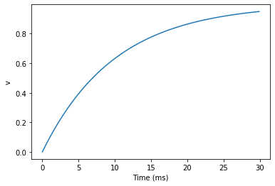
This time we only ran the simulation for 30 ms so that we can see the behaviour better. It looks like it’s behaving as expected, but let’s just check that analytically by plotting the expected behaviour on top.
start_scope()

G = NeuronGroup(1, eqs, method='exact')
M = StateMonitor(G, 'v', record=0)

run(30*ms)

plot(M.t/ms, M.v[0], 'C0', label='Brian')
plot(M.t/ms, 1-exp(-M.t/tau), 'C1--',label='Analytic')
xlabel('Time (ms)')
ylabel('v')
legend();
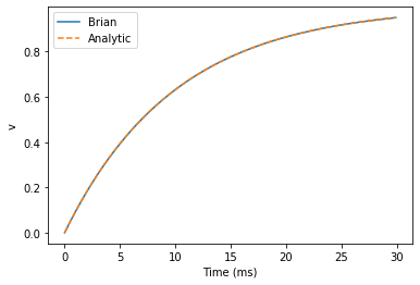
As you can see, the blue (Brian) and dashed orange (analytic solution) lines coincide.
In this example, we used the object StateMonitor object. This is
used to record the values of a neuron variable while the simulation
runs. The first two arguments are the group to record from, and the
variable you want to record from. We also specify record=0. This
means that we record all values for neuron 0. We have to specify which
neurons we want to record because in large simulations with many neurons
it usually uses up too much RAM to record the values of all neurons.
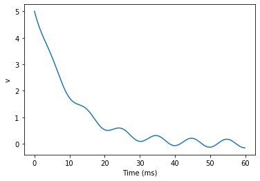
Now try modifying the equations and parameters and see what happens in the cell below.
start_scope()

tau = 10*ms
eqs = '''
dv/dt = (sin(2*pi*100*Hz*t)-v)/tau : 1
'''

# Change to Euler method because exact integrator doesn't work here
G = NeuronGroup(1, eqs, method='euler')
M = StateMonitor(G, 'v', record=0)

G.v = 5 # initial value

run(60*ms)

plot(M.t/ms, M.v[0])
xlabel('Time (ms)')
ylabel('v');
Adding spikes
So far we haven’t done anything neuronal, just played around with differential equations. Now let’s start adding spiking behaviour.
start_scope()

tau = 10*ms
eqs = '''
dv/dt = (1-v)/tau : 1
'''

G = NeuronGroup(1, eqs, threshold='v>0.8', reset='v = 0', method='exact')

M = StateMonitor(G, 'v', record=0)
run(50*ms)
plot(M.t/ms, M.v[0])
xlabel('Time (ms)')
ylabel('v');
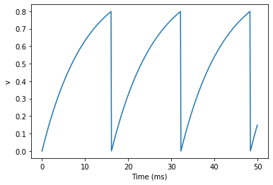
We’ve added two new keywords to the NeuronGroup declaration:
threshold='v>0.8' and reset='v = 0'. What this means is that
when v>0.8 we fire a spike, and immediately reset v = 0 after
the spike. We can put any expression and series of statements as these
strings.
As you can see, at the beginning the behaviour is the same as before
until v crosses the threshold v>0.8 at which point you see it
reset to 0. You can’t see it in this figure, but internally Brian has
registered this event as a spike. Let’s have a look at that.
start_scope()

G = NeuronGroup(1, eqs, threshold='v>0.8', reset='v = 0', method='exact')

spikemon = SpikeMonitor(G)

run(50*ms)

print('Spike times: %s' % spikemon.t[:])
Spike times: [16. 32.1 48.2] ms
The SpikeMonitor object takes the group whose spikes you want to
record as its argument and stores the spike times in the variable t.
Let’s plot those spikes on top of the other figure to see that it’s
getting it right.
start_scope()

G = NeuronGroup(1, eqs, threshold='v>0.8', reset='v = 0', method='exact')

statemon = StateMonitor(G, 'v', record=0)
spikemon = SpikeMonitor(G)

run(50*ms)

plot(statemon.t/ms, statemon.v[0])
for t in spikemon.t:
    axvline(t/ms, ls='--', c='C1', lw=3)
xlabel('Time (ms)')
ylabel('v');
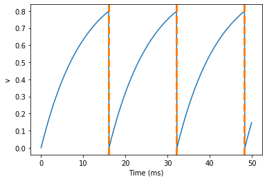
Here we’ve used the axvline command from matplotlib to draw an
orange, dashed vertical line at the time of each spike recorded by the
SpikeMonitor.
Now try changing the strings for threshold and reset in the cell
above to see what happens.
Refractoriness
A common feature of neuron models is refractoriness. This means that after the neuron fires a spike it becomes refractory for a certain duration and cannot fire another spike until this period is over. Here’s how we do that in Brian.
start_scope()

tau = 10*ms
eqs = '''
dv/dt = (1-v)/tau : 1 (unless refractory)
'''

G = NeuronGroup(1, eqs, threshold='v>0.8', reset='v = 0', refractory=5*ms, method='exact')

statemon = StateMonitor(G, 'v', record=0)
spikemon = SpikeMonitor(G)

run(50*ms)

plot(statemon.t/ms, statemon.v[0])
for t in spikemon.t:
    axvline(t/ms, ls='--', c='C1', lw=3)
xlabel('Time (ms)')
ylabel('v');
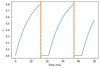
As you can see in this figure, after the first spike, v stays at 0
for around 5 ms before it resumes its normal behaviour. To do this,
we’ve done two things. Firstly, we’ve added the keyword
refractory=5*ms to the NeuronGroup declaration. On its own, this
only means that the neuron cannot spike in this period (see below), but
doesn’t change how v behaves. In order to make v stay constant
during the refractory period, we have to add (unless refractory) to
the end of the definition of v in the differential equations. What
this means is that the differential equation determines the behaviour of
v unless it’s refractory in which case it is switched off.
Here’s what would happen if we didn’t include (unless refractory).
Note that we’ve also decreased the value of tau and increased the
length of the refractory period to make the behaviour clearer.
start_scope()

tau = 5*ms
eqs = '''
dv/dt = (1-v)/tau : 1
'''

G = NeuronGroup(1, eqs, threshold='v>0.8', reset='v = 0', refractory=15*ms, method='exact')

statemon = StateMonitor(G, 'v', record=0)
spikemon = SpikeMonitor(G)

run(50*ms)

plot(statemon.t/ms, statemon.v[0])
for t in spikemon.t:
    axvline(t/ms, ls='--', c='C1', lw=3)
axhline(0.8, ls=':', c='C2', lw=3)
xlabel('Time (ms)')
ylabel('v')
print("Spike times: %s" % spikemon.t[:])
Spike times: [ 8. 23. 38.] ms
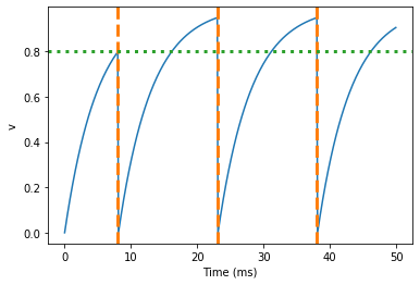
So what’s going on here? The behaviour for the first spike is the same:
v rises to 0.8 and then the neuron fires a spike at time 8 ms before
immediately resetting to 0. Since the refractory period is now 15 ms
this means that the neuron won’t be able to spike again until time 8 +
15 = 23 ms. Immediately after the first spike, the value of v now
instantly starts to rise because we didn’t specify
(unless refractory) in the definition of dv/dt. However, once it
reaches the value 0.8 (the dashed green line) at time roughly 8 ms it
doesn’t fire a spike even though the threshold is v>0.8. This is
because the neuron is still refractory until time 23 ms, at which point
it fires a spike.
Note that you can do more complicated and interesting things with refractoriness. See the full documentation for more details about how it works.
Multiple neurons
So far we’ve only been working with a single neuron. Let’s do something interesting with multiple neurons.
start_scope()

N = 100
tau = 10*ms
eqs = '''
dv/dt = (2-v)/tau : 1
'''

G = NeuronGroup(N, eqs, threshold='v>1', reset='v=0', method='exact')
G.v = 'rand()'

spikemon = SpikeMonitor(G)

run(50*ms)

plot(spikemon.t/ms, spikemon.i, '.k')
xlabel('Time (ms)')
ylabel('Neuron index');
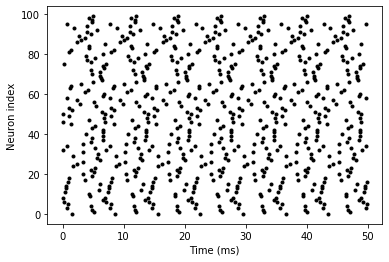
This shows a few changes. Firstly, we’ve got a new variable N
determining the number of neurons. Secondly, we added the statement
G.v = 'rand()' before the run. What this does is initialise each
neuron with a different uniform random value between 0 and 1. We’ve done
this just so each neuron will do something a bit different. The other
big change is how we plot the data in the end.
As well as the variable spikemon.t with the times of all the spikes,
we’ve also used the variable spikemon.i which gives the
corresponding neuron index for each spike, and plotted a single black
dot with time on the x-axis and neuron index on the y-value. This is the
standard “raster plot” used in neuroscience.
Parameters
To make these multiple neurons do something more interesting, let’s introduce per-neuron parameters that don’t have a differential equation attached to them.
start_scope()

N = 100
tau = 10*ms
v0_max = 3.
duration = 1000*ms

eqs = '''
dv/dt = (v0-v)/tau : 1 (unless refractory)
v0 : 1
'''

G = NeuronGroup(N, eqs, threshold='v>1', reset='v=0', refractory=5*ms, method='exact')
M = SpikeMonitor(G)

G.v0 = 'i*v0_max/(N-1)'

run(duration)

figure(figsize=(12,4))
subplot(121)
plot(M.t/ms, M.i, '.k')
xlabel('Time (ms)')
ylabel('Neuron index')
subplot(122)
plot(G.v0, M.count/duration)
xlabel('v0')
ylabel('Firing rate (sp/s)');
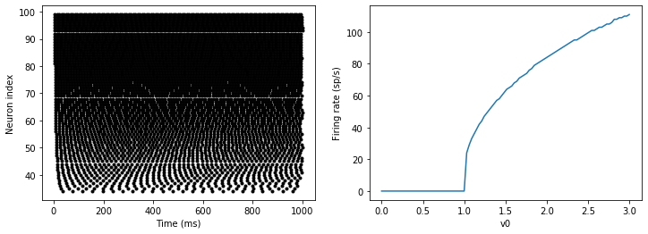
The line v0 : 1 declares a new per-neuron parameter v0 with
units 1 (i.e. dimensionless).
The line G.v0 = 'i*v0_max/(N-1)' initialises the value of v0 for
each neuron varying from 0 up to v0_max. The symbol i when it
appears in strings like this refers to the neuron index.
So in this example, we’re driving the neuron towards the value v0
exponentially, but when v crosses v>1, it fires a spike and
resets. The effect is that the rate at which it fires spikes will be
related to the value of v0. For v0<1 it will never fire a spike,
and as v0 gets larger it will fire spikes at a higher rate. The
right hand plot shows the firing rate as a function of the value of
v0. This is the I-f curve of this neuron model.
Note that in the plot we’ve used the count variable of the
SpikeMonitor: this is an array of the number of spikes each neuron
in the group fired. Dividing this by the duration of the run gives the
firing rate.
Stochastic neurons
Often when making models of neurons, we include a random element to
model the effect of various forms of neural noise. In Brian, we can do
this by using the symbol xi in differential equations. Strictly
speaking, this symbol is a “stochastic differential” but you can sort of
thinking of it as just a Gaussian random variable with mean 0 and
standard deviation 1. We do have to take into account the way stochastic
differentials scale with time, which is why we multiply it by
tau**-0.5 in the equations below (see a textbook on stochastic
differential equations for more details). Note that we also changed the
method keyword argument to use 'euler' (which stands for the
Euler-Maruyama
method);
the 'exact' method that we used earlier is not applicable to
stochastic differential equations.
start_scope()

N = 100
tau = 10*ms
v0_max = 3.
duration = 1000*ms
sigma = 0.2

eqs = '''
dv/dt = (v0-v)/tau+sigma*xi*tau**-0.5 : 1 (unless refractory)
v0 : 1
'''

G = NeuronGroup(N, eqs, threshold='v>1', reset='v=0', refractory=5*ms, method='euler')
M = SpikeMonitor(G)

G.v0 = 'i*v0_max/(N-1)'

run(duration)

figure(figsize=(12,4))
subplot(121)
plot(M.t/ms, M.i, '.k')
xlabel('Time (ms)')
ylabel('Neuron index')
subplot(122)
plot(G.v0, M.count/duration)
xlabel('v0')
ylabel('Firing rate (sp/s)');
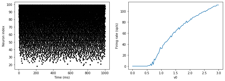
That’s the same figure as in the previous section but with some noise added. Note how the curve has changed shape: instead of a sharp jump from firing at rate 0 to firing at a positive rate, it now increases in a sigmoidal fashion. This is because no matter how small the driving force the randomness may cause it to fire a spike.
End of tutorial
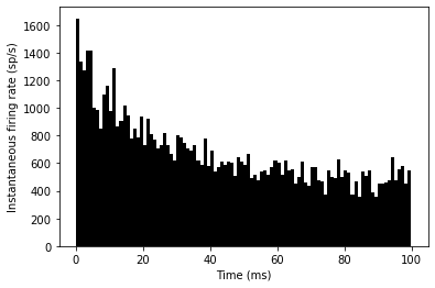
That’s the end of this part of the tutorial. The cell below has another
example. See if you can work out what it is doing and why. Try adding a
StateMonitor to record the values of the variables for one of the
neurons to help you understand it.
You could also try out the things you’ve learned in this cell.
Once you’re done with that you can move on to the next tutorial on Synapses.
start_scope()

N = 1000
tau = 10*ms
vr = -70*mV
vt0 = -50*mV
delta_vt0 = 5*mV
tau_t = 100*ms
sigma = 0.5*(vt0-vr)
v_drive = 2*(vt0-vr)
duration = 100*ms

eqs = '''
dv/dt = (v_drive+vr-v)/tau + sigma*xi*tau**-0.5 : volt
dvt/dt = (vt0-vt)/tau_t : volt
'''

reset = '''
v = vr
vt += delta_vt0
'''

G = NeuronGroup(N, eqs, threshold='v>vt', reset=reset, refractory=5*ms, method='euler')
spikemon = SpikeMonitor(G)

G.v = 'rand()*(vt0-vr)+vr'
G.vt = vt0

run(duration)

_ = hist(spikemon.t/ms, 100, histtype='stepfilled', facecolor='k', weights=list(ones(len(spikemon))/(N*defaultclock.dt)))
xlabel('Time (ms)')
ylabel('Instantaneous firing rate (sp/s)');