Example: Brette_Guigon_2003

Note

You can launch an interactive, editable version of this example without installing any local files using the Binder service (although note that at some times this may be slow or fail to open):

Reliability of spike timing

Adapted from Fig. 10D,E of

Brette R and E Guigon (2003). Reliability of Spike Timing Is a General Property of Spiking Model Neurons. Neural Computation 15, 279-308.

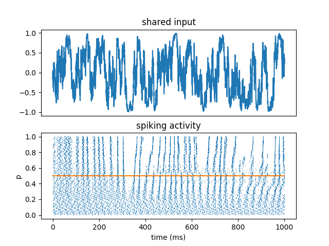
This shows that reliability of spike timing is a generic property of spiking neurons, even those that are not leaky. This is a non-physiological model which can be leaky or anti-leaky depending on the sign of the input I.

All neurons receive the same fluctuating input, scaled by a parameter p that varies across neurons. This shows:

1. reproducibility of spike timing

2. robustness with respect to deterministic changes (parameter)

3. increased reproducibility in the fluctuation-driven regime (input crosses the threshold)

from brian2 import *

N = 500
tau = 33*ms
taux = 20*ms
sigma = 0.02

eqs_input = '''
dx/dt = -x/taux + (2/taux)**.5*xi : 1
'''

eqs = '''
dv/dt = (v*I + 1)/tau + sigma*(2/tau)**.5*xi : 1
I = 0.5 + 3*p*B : 1
B = 2./(1 + exp(-2*x)) - 1 : 1 (shared)
p : 1
x : 1 (linked)
'''

input = NeuronGroup(1, eqs_input, method='euler')
neurons = NeuronGroup(N, eqs, threshold='v>1', reset='v=0', method='euler')
neurons.p = '1.0*i/N'
neurons.v = 'rand()'
neurons.x = linked_var(input, 'x')

M = StateMonitor(neurons, 'B', record=0)
S = SpikeMonitor(neurons)

run(1000*ms, report='text')

subplot(211)  # The input
plot(M.t/ms, M[0].B)
xticks([])
title('shared input')
subplot(212)
plot(S.t/ms, neurons.p[S.i], ',')
plot([0, 1000], [.5, .5], color='C1')
xlabel('time (ms)')
ylabel('p')
title('spiking activity')
show()