Example: efficient_gaussian_connectivity
Note
You can launch an interactive, editable version of this example without installing any local files using the Binder service (although note that at some times this may be slow or fail to open):
An example of turning an expensive Synapses.connect operation into
three cheap ones using a mathematical trick.
Consider the connection probability between neurons i and j given by the Gaussian function \(p=e^{-\alpha(i-j)^2}\) (for some constant \(\alpha\)). If we want to connect neurons with this probability, we can very simply do:
S.connect(p='exp(-alpha*(i-j)**2)')
However, this has a problem. Although we know that this will create
\(O(N)\) synapses if N is the number of neurons, because we
have specified p as a function of i and j, we have to evaluate
p(i, j) for every pair (i, j), and therefore it takes
\(O(N^2)\) operations.
Our first option is to take a cutoff, and say that if \(p<q\) for some
small \(q\), then we assume that \(p\approx 0\). We can work out
which j values are compatible with a given value of i by solving
\(e^{-\alpha(i-j)^2}<q\) which gives
\(|i-j|<\sqrt{-\log(q)/\alpha)}=w\). Now we implement the rule
using the generator syntax to only search for values between i-w
and i+w, except that some of these values will be outside the
valid range of values for j so we set skip_if_invalid=True.
The connection code is then:
S.connect(j='k for k in range(i-w, i+w) if rand()<exp(-alpha*(i-j)**2)',
          skip_if_invalid=True)
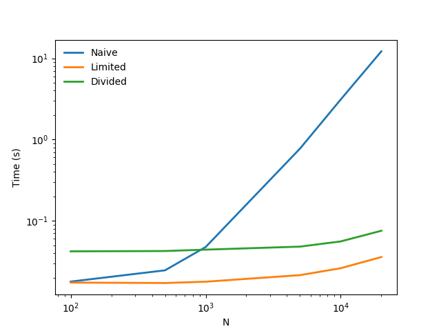
This is a lot faster (see graph labelled “Limited” for this algorithm).
However, it may be a problem that we have to specify a cutoff and so we will lose some synapses doing this: it won’t be mathematically exact. This isn’t a problem for the Gaussian because w grows very slowly with the cutoff probability q, but for other probability distributions with more weight in the tails, it could be an issue.
If we want to be exact, we can still do a big improvement. For the
case \(i-w\leq j\leq i+w\) we use the same connection code, but
we also handle the case \(|i-j|>w\). This time, we note that we
want to create a synapse with probability \(p(i-j)\) and we can
rewrite this as \(p(i-j)/p(w)\cdot p(w)\). If \(|i-j|>w\)
then this is a product of two probabilities \(p(i-j)/p(w)\)
and \(p(w)\). So in the region \(|i-j|>w\) a synapse
will be created if two random events both occur, with these
two probabilities. This might seem a little strange until you
notice that one of the two probabilities \(p(w)\) doesn’t
depend on i or j. This lets us use the much more efficient
sample algorithm to generate a set of candidate j values,
and then add the additional test rand()<p(i-j)/p(w). Here’s the
code for that:
w = int(ceil(sqrt(log(q)/-0.1)))
S.connect(j='k for k in range(i-w, i+w) if rand()<exp(-alpha*(i-j)**2)',
          skip_if_invalid=True)
pmax = exp(-0.1*w**2)
S.connect(j='k for k in sample(0, i-w, p=pmax) if rand()<exp(-alpha*(i-j)**2)/pmax',
          skip_if_invalid=True)
S.connect(j='k for k in sample(i+w, N_post, p=pmax) if rand()<exp(-alpha*(i-j)**2)/pmax',
          skip_if_invalid=True)
This “Divided” method is also much faster than the naive method, and is mathematically correct. Note though that this method is still \(O(N^2)\) but the constants are much, much smaller and this will usually be sufficient. It is possible to take the ideas developed here even further and get even better scaling, but in most cases it’s unlikely to be worth the effort.
The code below shows these examples written out, along with some timing code and plots for different values of N.
from brian2 import *
import time

def naive(N):
    G = NeuronGroup(N, 'v:1', threshold='v>1', name='G')
    S = Synapses(G, G, on_pre='v += 1', name='S')
    S.connect(p='exp(-0.1*(i-j)**2)')

def limited(N, q=0.001):
    G = NeuronGroup(N, 'v:1', threshold='v>1', name='G')
    S = Synapses(G, G, on_pre='v += 1', name='S')
    w = int(ceil(sqrt(log(q)/-0.1)))
    S.connect(j='k for k in range(i-w, i+w) if rand()<exp(-0.1*(i-j)**2)', skip_if_invalid=True)

def divided(N, q=0.001):
    G = NeuronGroup(N, 'v:1', threshold='v>1', name='G')
    S = Synapses(G, G, on_pre='v += 1', name='S')
    w = int(ceil(sqrt(log(q)/-0.1)))
    S.connect(j='k for k in range(i-w, i+w) if rand()<exp(-0.1*(i-j)**2)', skip_if_invalid=True)
    pmax = exp(-0.1*w**2)
    S.connect(j='k for k in sample(0, i-w, p=pmax) if rand()<exp(-0.1*(i-j)**2)/pmax', skip_if_invalid=True)
    S.connect(j='k for k in sample(i+w, N_post, p=pmax) if rand()<exp(-0.1*(i-j)**2)/pmax', skip_if_invalid=True)

def repeated_run(f, N, repeats):
    start_time = time.time()
    for _ in range(repeats):
        f(N)
    end_time = time.time()
    return (end_time-start_time)/repeats

N = array([100, 500, 1000, 5000, 10000, 20000])
repeats = array([100, 10, 10, 1, 1, 1])*3
naive(10)
limited(10)
divided(10)
print('Starting naive')
loglog(N, [repeated_run(naive, n, r) for n, r in zip(N, repeats)],
       label='Naive', lw=2)
print('Starting limit')
loglog(N, [repeated_run(limited, n, r) for n, r in zip(N, repeats)],
       label='Limited', lw=2)
print('Starting divided')
loglog(N, [repeated_run(divided, n, r) for n, r in zip(N, repeats)],
       label='Divided', lw=2)
xlabel('N')
ylabel('Time (s)')
legend(loc='best', frameon=False)
show()