Multicompartment models
It is possible to create neuron models with a spatially extended morphology, using
the SpatialNeuron class. A SpatialNeuron is a single neuron with many compartments.
Essentially, it works as a NeuronGroup where elements are compartments instead of neurons.
A SpatialNeuron is specified by a morphology (see Creating a neuron morphology) and a set of equations for
transmembrane currents (see Creating a spatially extended neuron).
Creating a neuron morphology
Schematic morphologies
Morphologies can be created combining geometrical objects:
soma = Soma(diameter=30*um)
cylinder = Cylinder(diameter=1*um, length=100*um, n=10)
The first statement creates a single iso-potential compartment (i.e. with no axial resistance within the compartment), with its area calculated as the area of a sphere with the given diameter. The second one specifies a cylinder consisting of 10 compartments with identical diameter and the given total length.
For more precise control over the geometry, you can specify the length and diameter of each individual compartment,
including the diameter at the start of the section (i.e. for n compartments: n length and n+1 diameter
values) in a Section object:
section = Section(diameter=[6, 5, 4, 3, 2, 1]*um, length=[10, 10, 10, 5, 5]*um, n=5)
The individual compartments are modeled as truncated cones, changing the diameter linearly between the given diameters
over the length of the compartment. Note that the diameter argument specifies the values at the nodes between the
compartments, but accessing the diameter attribute of a Morphology object will return the diameter at the center
of the compartment (see the note below).
The following table summarizes the different options to create schematic morphologies (the black compartment before the start of the section represents the parent compartment with diameter 15 μm, not specified in the code below):
| Example | |
|---|---|
| Soma |
 |
| Cylinder |
 |
| Section |
 |
Note
For a Section, the diameter argument specifies the diameter between the compartments
(and at the beginning/end of the first/last compartment). the corresponding values can therefore be later retrieved
from the Morphology via the start_diameter and end_diameter attributes. The diameter attribute of a
Morphology does correspond to the diameter at the midpoint of the compartment. For a Cylinder,
start_diameter, diameter, and end_diameter are of course all identical.
The tree structure of a morphology is created by attaching Morphology objects together:
morpho = Soma(diameter=30*um)
morpho.axon = Cylinder(length=100*um, diameter=1*um, n=10)
morpho.dendrite = Cylinder(length=50*um, diameter=2*um, n=5)
These statements create a morphology consisting of a cylindrical axon and a dendrite attached to a spherical soma.
Note that the names axon and dendrite are arbitrary and chosen by the user. For example, the same morphology can
be created as follows:
morpho = Soma(diameter=30*um)
morpho.output_process = Cylinder(length=100*um, diameter=1*um, n=10)
morpho.input_process = Cylinder(length=50*um, diameter=2*um, n=5)
The syntax is recursive, for example two sections can be added at the end of the dendrite as follows:
morpho.dendrite.branch1 = Cylinder(length=50*um, diameter=1*um, n=3)
morpho.dendrite.branch2 = Cylinder(length=50*um, diameter=1*um, n=3)
Equivalently, one can use an indexing syntax:
morpho['dendrite']['branch1'] = Cylinder(length=50*um, diameter=1*um, n=3)
morpho['dendrite']['branch2'] = Cylinder(length=50*um, diameter=1*um, n=3)
The names given to sections are completely up to the user. However, names that consist of a single digit (1 to
9) or the letters L (for left) and R (for right) allow for a special short syntax: they can be joined
together directly, without the needs for dots (or dictionary syntax) and therefore allow to quickly navigate through
the morphology tree (e.g. morpho.LRLLR is equivalent to morpho.L.R.L.L.R). This short syntax can also be used to
create trees:
morpho = Soma(diameter=30*um)
morpho.L = Cylinder(length=10*um, diameter=1*um, n=3)
morpho.L1 = Cylinder(length=5*um, diameter=1*um, n=3)
morpho.L2 = Cylinder(length=5*um, diameter=1*um, n=3)
morpho.L3 = Cylinder(length=5*um, diameter=1*um, n=3)
morpho.R = Cylinder(length=10*um, diameter=1*um, n=3)
morpho.RL = Cylinder(length=5*um, diameter=1*um, n=3)
morpho.RR = Cylinder(length=5*um, diameter=1*um, n=3)
The above instructions create a dendritic tree with two main sections, three sections attached to the first section and
two to the second. This can be verified with the Morphology.topology() method:
>>> morpho.topology()
( )  [root]
   `---|  .L
        `---|  .L.1
        `---|  .L.2
        `---|  .L.3
   `---|  .R
        `---|  .R.L
        `---|  .R.R
Note that an expression such as morpho.L will always refer to the entire subtree. However, accessing the attributes
(e.g. diameter) will only return the values for the given section.
Note
To avoid ambiguities, do not use names for sections that can be interpreted in the abbreviated way detailed above.
For example, do not name a child section L1 (which will be interpreted as the first child of the child L)
The number of compartments in a section can be accessed with morpho.n (or morpho.L.n, etc.), the number of
total sections and compartments in a subtree can be accessed with morpho.total_sections and
morpho.total_compartments respectively.
Adding coordinates
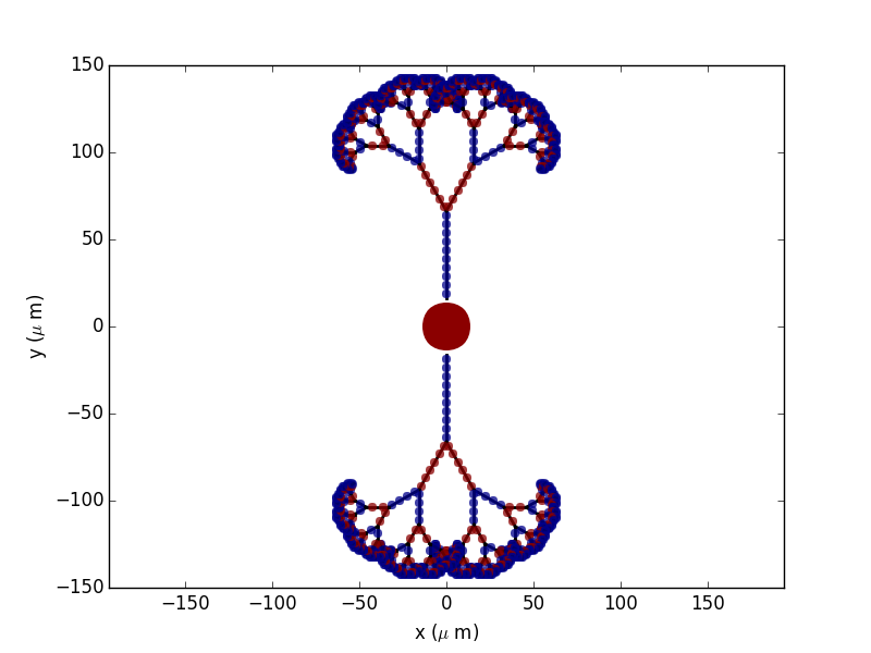
For plotting purposes, it can be useful to add coordinates to a Morphology that was created using the “schematic”
approach described above. This can be done by calling the generate_coordinates method on a morphology,
which will return an identical morphology but with additional 2D or 3D coordinates. By default, this method creates a
morphology according to a deterministic algorithm in 2D:
new_morpho = morpho.generate_coordinates()
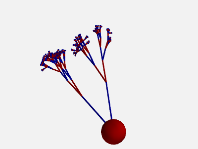
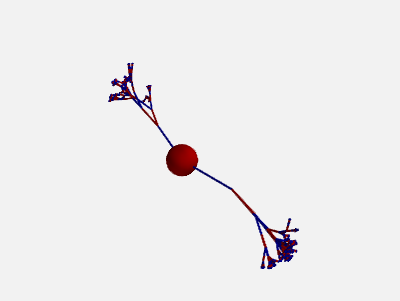
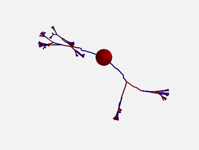
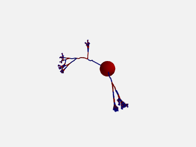
To get more “realistic” morphologies, this function can also be used to create morphologies in 3D where the orientation of each section differs from the orientation of the parent section by a random amount:
new_morpho = morpho.generate_coordinates(section_randomness=25)
|
|
|
This algorithm will base the orientation of each section on the orientation of the parent section and then randomly
perturb this orientation. More precisely, the algorithm first chooses a random vector orthogonal to the orientation
of the parent section. Then, the section will be rotated around this orthogonal vector by a random angle, drawn from an
exponential distribution with the \(\beta\) parameter (in degrees) given by section_randomness. This
\(\beta\) parameter specifies both the mean and the standard deviation of the rotation angle. Note that no maximum
rotation angle is enforced, values for section_randomness should therefore be reasonably small (e.g. using a
section_randomness of 45 would already lead to a probability of ~14% that the section will be rotated by more
than 90 degrees, therefore making the section go “backwards”).
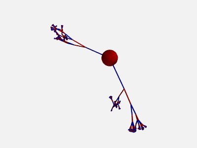
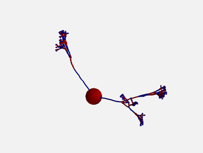
In addition, also the orientation of each compartment within a section can be randomly varied:
new_morpho = morpho.generate_coordinates(section_randomness=25,
                                         compartment_randomness=15)
|
|
|
The algorithm is the same as the one presented above, but applied individually to each compartment within a section (still based on the orientation on the parent section, not on the orientation of the previous compartment).
Complex morphologies
Morphologies can also be created from information about the compartment coordinates in 3D space. Such morphologies can
be loaded from a .swc file (a standard format for neuronal morphologies; for a large database of morphologies in
this format see http://neuromorpho.org):
morpho = Morphology.from_file('corticalcell.swc')
To manually create a morphology from a list of points in a similar format to SWC files, see Morphology.from_points.
Morphologies that are created in such a way will use standard names for the sections that allow for the short syntax
shown in the previous sections: if a section has one or two child sections, then they will be called L and R,
otherwise they will be numbered starting at 1.
Morphologies with coordinates can also be created section by section, following the same syntax as for “schematic” morphologies:
soma = Soma(diameter=30*um, x=50*um, y=20*um)
cylinder = Cylinder(n=10, x=[0, 100]*um, diameter=1*um)
section = Section(n=5,
                  x=[0, 10, 20, 30, 40, 50]*um,
                  y=[0, 10, 20, 30, 40, 50]*um,
                  z=[0, 10, 10, 10, 10, 10]*um,
                  diameter=[6, 5, 4, 3, 2, 1]*um)
Note that the x, y, z attributes of Morphology and SpatialNeuron will return the coordinates at the
midpoint of each compartment (as for all other attributes that vary over the length of a compartment, e.g. diameter
or distance), but during construction the coordinates refer to the start and end of the section (Cylinder),
respectively to the coordinates of the nodes between the compartments (Section).
A few additional remarks:
- In the majority of simulations, coordinates are not used in the neuronal equations, therefore the coordinates are purely for visualization purposes and do not affect the simulation results in any way.
- Coordinate specification cannot be combined with length specification – lengths are automatically calculated from the coordinates.
- The coordinate specification can also be 1- or 2-dimensional (as in the first two examples above), the unspecified coordinate will use 0 μm.
- All coordinates are interpreted relative to the parent compartment, i.e. the point (0 μm, 0 μm, 0 μm) refers to the
end point of the previous compartment. Most of the time, the first element of the coordinate specification is
therefore 0 μm, to continue a section where the previous one ended. However, it can be convenient to use a value
different from 0 μm for sections connecting to the
Somato make them (visually) connect to a point on the sphere surface instead of the center of the sphere.
Creating a spatially extended neuron
A SpatialNeuron is a spatially extended neuron. It is created by specifying the morphology as a
Morphology object, the equations for transmembrane currents, and optionally the specific membrane capacitance
Cm and intracellular resistivity Ri:
gL = 1e-4*siemens/cm**2
EL = -70*mV
eqs = '''
Im=gL * (EL - v) : amp/meter**2
I : amp (point current)
'''
neuron = SpatialNeuron(morphology=morpho, model=eqs, Cm=1*uF/cm**2, Ri=100*ohm*cm)
neuron.v = EL + 10*mV
Several state variables are created automatically: the SpatialNeuron inherits all the geometrical variables of the
compartments (length, diameter, area, volume), as well as the distance variable that gives the
distance to the soma. For morphologies that use coordinates, the x, y and z variables are provided as well.
Additionally, a state variable Cm is created. It is initialized with the value given at construction, but it can be
modified on a compartment per compartment basis (which is useful to model myelinated axons). The membrane potential is
stored in state variable v.
Note that for all variable values that vary across a compartment (e.g. distance, x, y, z, v), the
value that is reported is the value at the midpoint of the compartment.
The key state variable, which must be specified at construction, is Im. It is the total transmembrane current,
expressed in units of current per area. This is a mandatory line in the definition of the model. The rest of the
string description may include other state variables (differential equations or subexpressions)
or parameters, exactly as in NeuronGroup. At every timestep, Brian integrates the state variables, calculates the
transmembrane current at every point on the neuronal morphology, and updates v using the transmembrane current and
the diffusion current, which is calculated based on the morphology and the intracellular resistivity.
Note that the transmembrane current is a surfacic current, not the total current in the compartement.
This choice means that the model equations are independent of the number of compartments chosen for the simulation.
The space and time constants can obtained for any point of the neuron with the space_constant respectively
time_constant attributes:
l = neuron.space_constant[0]
tau = neuron.time_constant[0]
The calculation is based on the local total conductance (not just the leak conductance), therefore, it can potentially vary during a simulation (e.g. decrease during an action potential). The reported value is only correct for compartments with a cylindrical geometry, though, it does not give reasonable values for compartments with strongly varying diameter.
To inject a current I at a particular point (e.g. through an electrode or a synapse), this current must be divided by
the area of the compartment when inserted in the transmembrane current equation. This is done automatically when
the flag point current is specified, as in the example above. This flag can apply only to subexpressions or
parameters with amp units. Internally, the expression of the transmembrane current Im is simply augmented with
+I/area. A current can then be injected in the first compartment of the neuron (generally the soma) as follows:
neuron.I[0] = 1*nA
State variables of the SpatialNeuron include all the compartments of that neuron (including subtrees).
Therefore, the statement neuron.v = EL + 10*mV sets the membrane potential of the entire neuron at -60 mV.
Subtrees can be accessed by attribute (in the same way as in Morphology objects):
neuron.axon.gNa = 10*gL
Note that the state variables correspond to the entire subtree, not just the main section.
That is, if the axon had branches, then the above statement would change gNa on the main section
and all the sections in the subtree. To access the main section only, use the attribute main:
neuron.axon.main.gNa = 10*gL
A typical use case is when one wants to change parameter values at the soma only. For example, inserting an electrode current at the soma is done as follows:
neuron.main.I = 1*nA
A part of a section can be accessed as follows:
initial_segment = neuron.axon[10*um:50*um]
Synaptic inputs
There are two methods to have synapses on SpatialNeuron.
The first one to insert synaptic equations directly in the neuron equations:
eqs='''
Im = gL * (EL - v) : amp/meter**2
Is = gs * (Es - v) : amp (point current)
dgs/dt = -gs/taus : siemens
'''
neuron = SpatialNeuron(morphology=morpho, model=eqs, Cm=1*uF/cm**2, Ri=100*ohm*cm)
Note that, as for electrode stimulation, the synaptic current must be defined as a point current.
Then we use a Synapses object to connect a spike source to the neuron:
S = Synapses(stimulation, neuron, on_pre='gs += w')
S.connect(i=0, j=50)
S.connect(i=1, j=100)
This creates two synapses, on compartments 50 and 100. One can specify the compartment number with its spatial position by indexing the morphology:
S.connect(i=0, j=morpho[25*um])
S.connect(i=1, j=morpho.axon[30*um])
In this method for creating synapses,
there is a single value for the synaptic conductance in any compartment.
This means that it will fail if there are several synapses onto the same compartment and synaptic equations
are nonlinear.
The second method, which works in such cases, is to have synaptic equations in the
Synapses object:
eqs='''
Im = gL * (EL - v) : amp/meter**2
Is = gs * (Es - v) : amp (point current)
gs : siemens
'''
neuron = SpatialNeuron(morphology=morpho, model=eqs, Cm=1 * uF / cm ** 2, Ri=100 * ohm * cm)
S = Synapses(stimulation, neuron, model='''dg/dt = -g/taus : siemens
                                           gs_post = g : siemens (summed)''',
             on_pre='g += w')
Here each synapse (instead of each compartment) has an associated value g, and all values of
g for each compartment (i.e., all synapses targeting that compartment) are collected
into the compartmental variable gs.
Detecting spikes
To detect and record spikes, we must specify a threshold condition, essentially in the same
way as for a NeuronGroup:
neuron = SpatialNeuron(morphology=morpho, model=eqs, threshold='v > 0*mV', refractory='v > -10*mV')
Here spikes are detected when the membrane potential v reaches 0 mV. Because there is generally
no explicit reset in this type of model (although it is possible to specify one), v remains above
0 mV for some time. To avoid detecting spikes during this entire time, we specify a refractory period.
In this case no spike is detected as long as v is greater than -10 mV. Another possibility could be:
neuron = SpatialNeuron(morphology=morpho, model=eqs, threshold='m > 0.5', refractory='m > 0.4')
where m is the state variable for sodium channel activation (assuming this has been defined in the
model). Here a spike is detected when half of the sodium channels are open.
With the syntax above, spikes are detected in all compartments of the neuron. To detect them in a single
compartment, use the threshold_location keyword:
neuron = SpatialNeuron(morphology=morpho, model=eqs, threshold='m > 0.5', threshold_location=30,
                       refractory='m > 0.4')
In this case, spikes are only detecting in compartment number 30. Reset then applies locally to that compartment (if a reset statement is defined). Again the location of the threshold can be specified with spatial position:
neuron = SpatialNeuron(morphology=morpho, model=eqs, threshold='m > 0.5',
                       threshold_location=morpho.axon[30*um],
                       refractory='m > 0.4')